How to Structure Your Code for Statistical Consultations

Author

Allen Bush-Beaupré

Introduction

This document provides a template for structuring your R code when sharing analyses for statistical consultation. A well-organized document helps me understand your research question, data, and analysis quickly, allowing me to provide better feedback.

Key Elements of Good Code Structure:

Clear introduction stating your research question
Load packages at the beginning
Data exploration before analysis
Commented code explaining your thinking
Interpret results in plain language

What are Quarto and R Markdown?

Quarto and R Markdown are document formats that combine text (like a Word document) with executable R code. They’re perfect for reproducible analyses because:

Your code and explanations live in the same document
You can re-run analyses with one click
Outputs (plots, tables, statistics) are automatically updated
You can share as HTML, PDF, or Word documents

Quarto vs R Markdown - Which Should I Use?

Both work great! The main differences:

R Markdown (.Rmd): The older, well-established format - requires rmarkdown package
Quarto (.qmd): The newer format - works with R, Python, Julia, and more - doesn’t require extra R packages

For consultations, either format is fine! Use whichever you’re comfortable with.

How to Create a Quarto/R Markdown Document

In RStudio:

File → New File → Quarto Document (or R Markdown)
Give it a title and author
Choose HTML as output format
Click “Create”

How to Render to HTML

Once you’ve written your document, you need to “render” it to create the HTML output:

Method 1: Click the Render/Knit button - Quarto: Click the “Render” button at the top of the editor - R Markdown: Click the “Knit” button at the top of the editor

Method 2: Use the console

# For Quarto documents (.qmd)
quarto::quarto_render("your_file.qmd")

# For R Markdown documents (.Rmd)
rmarkdown::render("your_file.Rmd")

Method 3: Use the terminal

# For Quarto documents
quarto render your_file.qmd

What to Send Me

When sharing your analysis for consultation, please send me both:

The source file (.qmd or .Rmd) - so I can see your code
The rendered HTML (.html) - so I can view your results without running the code

This way, I can review your outputs and dive into your code if needed!

Basic Document Structure

Here’s a minimal template to get you started:

---
title: "My Analysis Title"
author: "Your Name"
date: "2026-01-12"
format: html
---

## Introduction

What is your research question?

## Load Packages

```{r}
library(tidyverse)
```

## Load Data

```{r}
my_data <- read_csv("data.csv")
```

## Analysis

```{r}
# Your analysis code here
```

## Results

What do your results mean?

Example: Fiddler Crab Analysis

Let’s explore whether fiddler crabs follow Bergmann’s Rule - the pattern where organisms at higher latitudes are larger than those at lower latitudes.

Research Question

Do Atlantic marsh fiddler crabs (Minuca pugnax) show larger body sizes at higher latitudes along the US Atlantic coast?

Load Required Packages

library(lterdatasampler)  # Contains the pie_crab dataset
library(tidyverse)         # For data manipulation and visualization
library(broom)            # For tidy model outputs

Load and Explore the Data

# View the first few rows
head(pie_crab)

# A tibble: 6 × 9
  date       latitude site   size air_temp air_temp_sd water_temp water_temp_sd
  <date>        <dbl> <chr> <dbl>    <dbl>       <dbl>      <dbl>         <dbl>
1 2016-07-24       30 GTM    12.4     21.8        6.39       24.5          6.12
2 2016-07-24       30 GTM    14.2     21.8        6.39       24.5          6.12
3 2016-07-24       30 GTM    14.5     21.8        6.39       24.5          6.12
4 2016-07-24       30 GTM    12.9     21.8        6.39       24.5          6.12
5 2016-07-24       30 GTM    12.4     21.8        6.39       24.5          6.12
6 2016-07-24       30 GTM    13.0     21.8        6.39       24.5          6.12
# ℹ 1 more variable: name <chr>

# Check structure
str(pie_crab)

tibble [392 × 9] (S3: tbl_df/tbl/data.frame)
 $ date         : Date[1:392], format: "2016-07-24" "2016-07-24" ...
 $ latitude     : num [1:392] 30 30 30 30 30 30 30 30 30 30 ...
 $ site         : chr [1:392] "GTM" "GTM" "GTM" "GTM" ...
 $ size         : num [1:392] 12.4 14.2 14.5 12.9 12.4 ...
 $ air_temp     : num [1:392] 21.8 21.8 21.8 21.8 21.8 ...
 $ air_temp_sd  : num [1:392] 6.39 6.39 6.39 6.39 6.39 ...
 $ water_temp   : num [1:392] 24.5 24.5 24.5 24.5 24.5 ...
 $ water_temp_sd: num [1:392] 6.12 6.12 6.12 6.12 6.12 ...
 $ name         : chr [1:392] "Guana Tolomoto Matanzas NERR" "Guana Tolomoto Matanzas NERR" "Guana Tolomoto Matanzas NERR" "Guana Tolomoto Matanzas NERR" ...

# Summary statistics
summary(pie_crab)

      date               latitude         site                size      
 Min.   :2016-07-24   Min.   :30.00   Length:392         Min.   : 6.64  
 1st Qu.:2016-07-28   1st Qu.:34.00   Class :character   1st Qu.:12.02  
 Median :2016-08-01   Median :39.10   Mode  :character   Median :14.44  
 Mean   :2016-08-02   Mean   :37.69                      Mean   :14.66  
 3rd Qu.:2016-08-09   3rd Qu.:41.60                      3rd Qu.:17.34  
 Max.   :2016-08-13   Max.   :42.70                      Max.   :23.43  
    air_temp      air_temp_sd      water_temp    water_temp_sd  
 Min.   :10.29   Min.   :6.391   Min.   :13.98   Min.   :4.838  
 1st Qu.:12.05   1st Qu.:8.110   1st Qu.:14.33   1st Qu.:6.567  
 Median :13.93   Median :8.410   Median :17.50   Median :6.998  
 Mean   :15.20   Mean   :8.654   Mean   :17.65   Mean   :7.252  
 3rd Qu.:18.63   3rd Qu.:9.483   3rd Qu.:20.54   3rd Qu.:7.865  
 Max.   :21.79   Max.   :9.965   Max.   :24.50   Max.   :9.121  
     name          
 Length:392        
 Class :character  
 Mode  :character

Data Exploration: Visualize Relationships

Before running statistical tests, always visualize your data!

Relationship between latitude and water temperature

ggplot(data = pie_crab, aes(x = water_temp, y = latitude)) +
  geom_point() +
  labs(x = "Water Temperature (°C)",
       y = "Latitude",
       title = "Water temperature decreases at higher latitudes") +
  theme_minimal()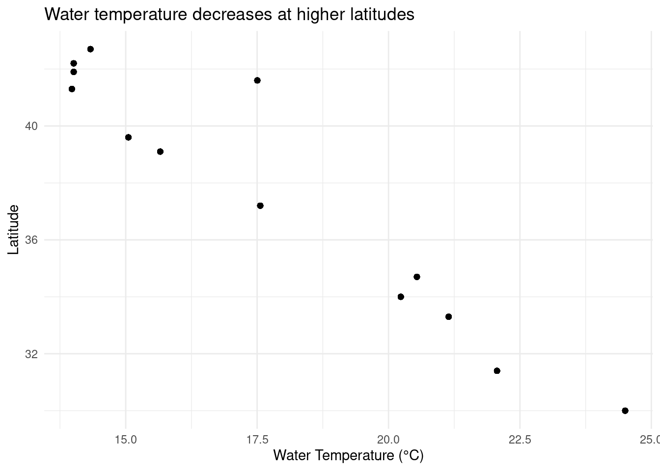

Crab size distribution by latitude

ggplot(data = pie_crab, aes(x = size, y = latitude, group = latitude)) +
  geom_boxplot(aes(color = latitude)) +
  labs(x = "Carapace Width (mm)",
       y = "Latitude",
       title = "Fiddler crab size appears to increase with latitude") +
  theme_minimal() +
  theme(legend.position = "none")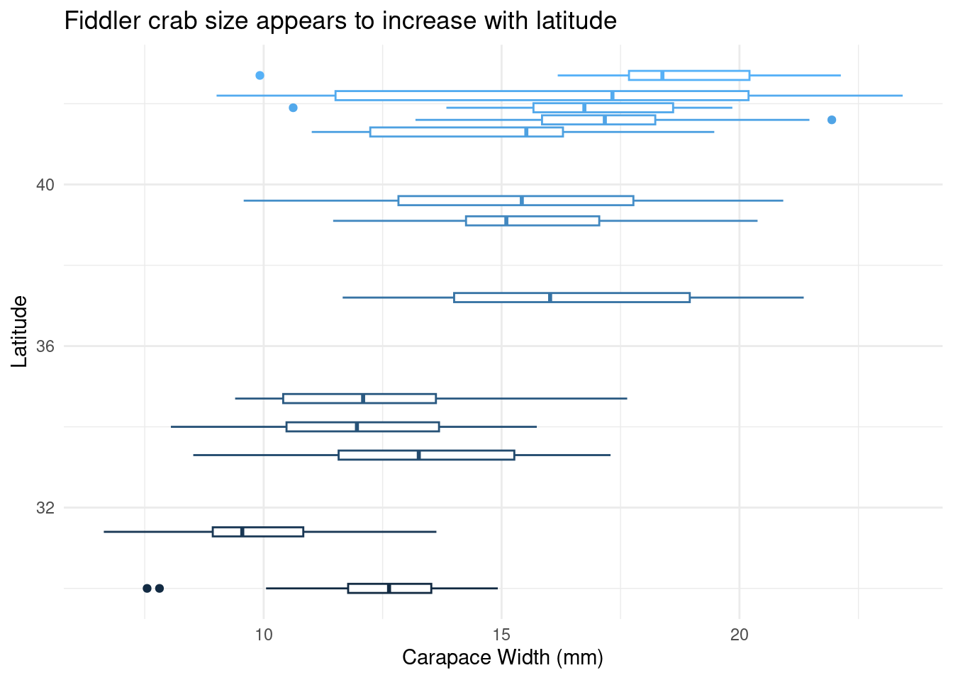

Observation: The boxplots suggest that crab size increases at higher latitudes, consistent with Bergmann’s Rule.

Statistical Analysis

Simple Linear Regression

Testing if latitude predicts crab size:

# Fit the model
crab_model <- lm(size ~ latitude, data = pie_crab)

# View results
summary(crab_model)


Call:
lm(formula = size ~ latitude, data = pie_crab)

Residuals:
    Min      1Q  Median      3Q     Max 
-7.8376 -1.8797  0.1144  1.9484  6.9280 

Coefficients:
            Estimate Std. Error t value Pr(>|t|)    
(Intercept) -3.62442    1.27405  -2.845  0.00468 ** 
latitude     0.48512    0.03359  14.441  < 2e-16 ***
---
Signif. codes:  0 '***' 0.001 '**' 0.01 '*' 0.05 '.' 0.1 ' ' 1

Residual standard error: 2.832 on 390 degrees of freedom
Multiple R-squared:  0.3484,    Adjusted R-squared:  0.3467 
F-statistic: 208.5 on 1 and 390 DF,  p-value: < 2.2e-16

# Tidy output (optional but nice!)
tidy(crab_model)

# A tibble: 2 × 5
  term        estimate std.error statistic  p.value
  <chr>          <dbl>     <dbl>     <dbl>    <dbl>
1 (Intercept)   -3.62     1.27       -2.84 4.68e- 3
2 latitude       0.485    0.0336     14.4  3.60e-38

Model Diagnostics

Always check your model assumptions!

par(mfrow = c(2, 2))  # 2x2 plot layout
plot(crab_model)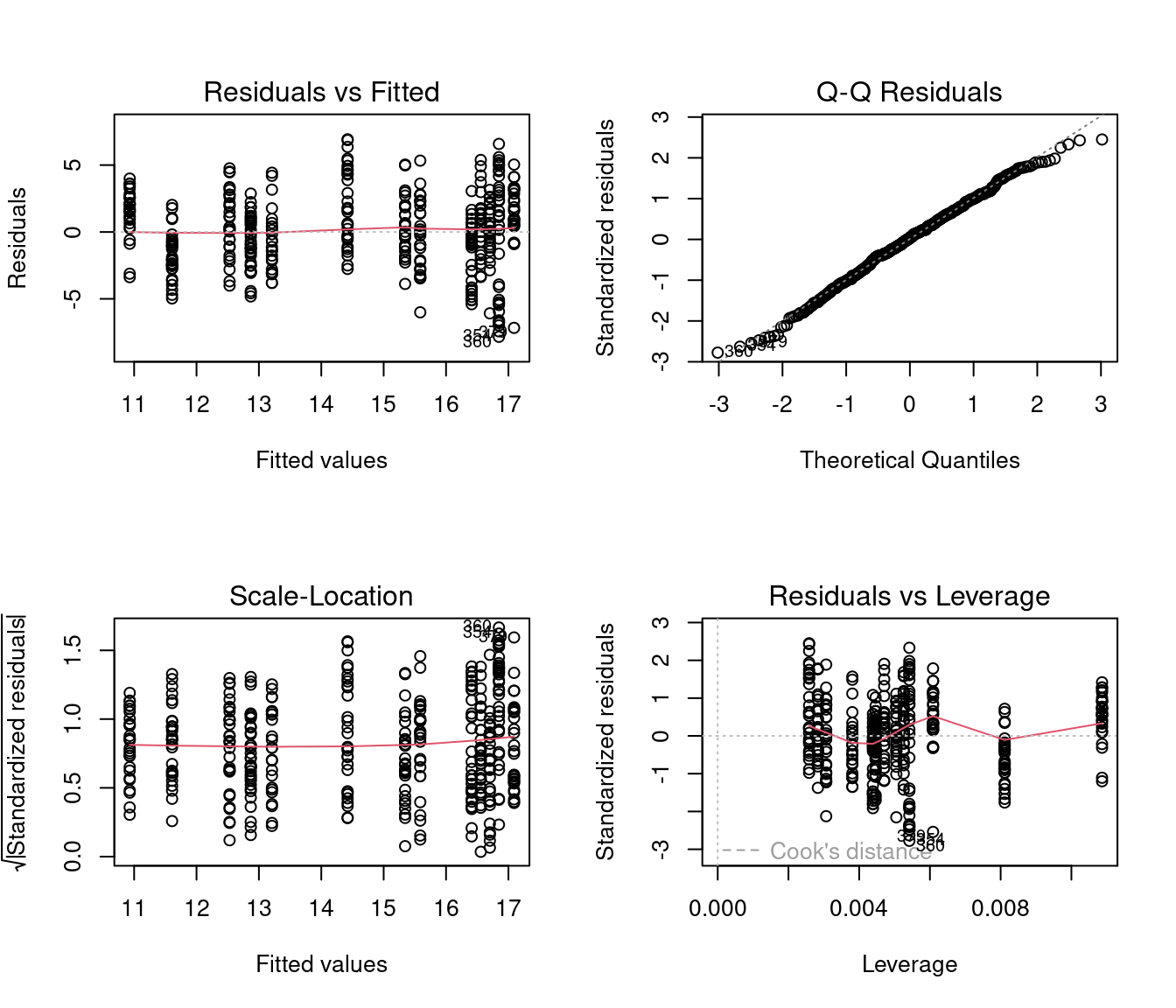

Results Interpretation

# Extract key statistics
model_stats <- glance(crab_model)
coef_stats <- tidy(crab_model)

# Print in plain language
cat("Model Results:\n")

Model Results:

cat("- Slope:", round(coef_stats$estimate[2], 3), "mm per degree latitude\n")

- Slope: 0.485 mm per degree latitude

cat("- P-value:", format(coef_stats$p.value[2], scientific = TRUE), "\n")

- P-value: 3.602897e-38

cat("- R-squared:", round(model_stats$r.squared, 3), "\n")

- R-squared: 0.348

Interpretation: For each 1-degree increase in latitude, crab carapace width increases by approximately 0.49 mm on average (p < 0.001). Latitude explains about 35% of the variation in crab size. This supports Bergmann’s Rule for this species.

Conclusions

Fiddler crabs show larger body sizes at higher latitudes along the US Atlantic coast
The relationship is statistically significant (p < 0.001)
However, latitude only explains ~35% of size variation - other factors likely matter
Model diagnostics look reasonable (residuals appear normally distributed)

Next Steps (Optional)

If I were to extend this analysis, I would:

Test for non-linear relationships (e.g., quadratic terms)
Include water temperature as a predictor
Check for site-level effects (mixed models)
Examine if the temperature-size rule applies

Tips for Your Own Code

✅ DO:

Start with a clear research question
Load all packages at the top
Comment your code liberally
Visualize before analyzing
Check model assumptions
Interpret results in plain language

❌ DON’T:

Run analyses without exploring the data first
Forget to check model diagnostics
Leave code without comments
Skip interpretation of statistical outputs
Send code that doesn’t run!