Visualizing indirect effects – Allen Bush-Beaupré

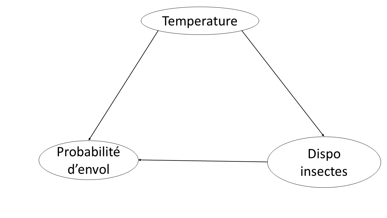
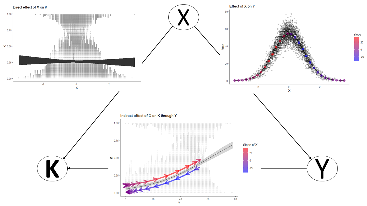
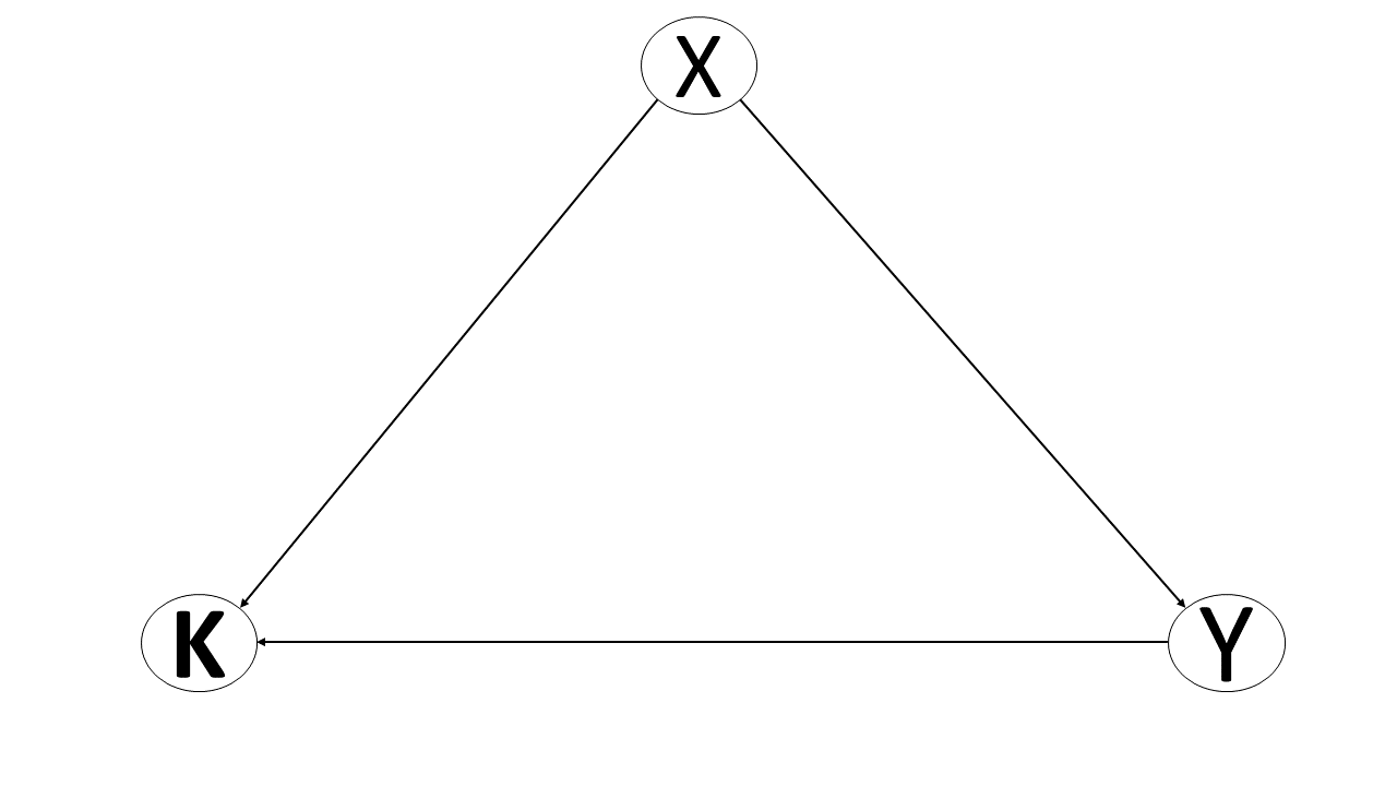
When fitting a model (ex. glm) in a causal inference context, we are either estimating the direct or total effect of a given variable. For example, in a DAG such as this one:

We can estimate the direct effect of X on K by fitting a model such as

lm(K ~ X + Y)

In this case, we estimate the direct effect of X on K as we are controlling for Y. Such is the nature of (generalized) linear models.

If we want to estimate the total effect of X on K, we simply fit the model

lm(K ~ X)

In this case, as we are ignoring Y, we estimate the direct effect of X + its indirect effect through Y (the total effect).

But what if we are interested in looking at the indirect effects?

As François Briau once told me, the study of Ecology is the study of direct and indirect effects. We just don’t really do it formally.

Luckily, Bill Shipley has spent quite a bit of brain power in quantifying direct, indirect and total effects which is what we call Path Analysis.

Very briefly, to calculate indirect effects in along a path (ex. TSF -> Sphagnum cover -> forest floor thickness), one must multiply the (standardized) coefficients along that path. In this case, 0.073 * 0.164 = 0.011972

N. Fenton et al. / Forest Ecology and Management 213 (2005) 151–159

But what does that number represent? When all relationships are linear, that value represents a slope. When the relationship(s) is/are not linear (ex. Poisson and logistic regressions), the value represents the slope on the link scale (log or logit or other). On the response scale, the slope is not constant through the entire relationship (we will see later). So how do we interpret such indirect effects if they are not on the scale of the variable we measured?

Start by loading the pertinent packages

Code

rm(list=ls()) # clear workspace
library(tidyverse) # data manipulation and plotting
library(glmmTMB) # frequentist glmms
library(patchwork) #multiple plots
library(ggdist) # nice dots in logistic regression
library(tidylog) # log changes done during data wrangling
library(mgcv) # gamms
library(gratia) # gam predictions

First, we will simulate data from this DAG:

But these are just letters - BORING

The DAG could also be

You don`t have to think too hard to see this type of relationship in your own work.

Code

set.seed(333) # set seed to reproduce the simulations exactly
n <- 3000 # sample size
X <- rnorm(n, 0, 1) # define K as a Z-score
Y <- rpois(n, exp(4 + 0.5*X)) # Y is a poisson variable whose link is the log function so defining the coefficients using the inverse log (exponential)
K <- rbinom(n, size = 1, prob = plogis(-3 + 0.03*X + 0.05*Y)) # K is a Bernoulli variable whose link is the logit so defining the coefficients using the inverse logit (plogis)

data <- tibble(
  X = X,
  Y = Y,
  K = K,
  K_1 = 1 - K
)

head(data)

# A tibble: 6 × 4
        X     Y     K   K_1
    <dbl> <int> <int> <dbl>
1 -0.0828    42     0     1
2  1.93     151     1     0
3 -2.05      20     0     1
4  0.278     65     0     1
5 -1.53      22     0     1
6 -0.269     56     0     1

Now, we want to model this path analysis

Model for Y

Code

mY_X <- glmmTMB(Y ~ X, family = poisson, data = data)
summary(mY_X)

 Family: poisson  ( log )
Formula:          Y ~ X
Data: data

      AIC       BIC    logLik -2*log(L)  df.resid 
  20576.1   20588.1  -10286.1   20572.1      2998 


Conditional model:
            Estimate Std. Error z value Pr(>|z|)    
(Intercept) 3.997055   0.002606    1534   <2e-16 ***
X           0.499396   0.002281     219   <2e-16 ***
---
Signif. codes:  0 '***' 0.001 '**' 0.01 '*' 0.05 '.' 0.1 ' ' 1

Model for K

Code

mK_XY <- glmmTMB(cbind(K, K_1) ~ X + Y, family = binomial, data = data)
summary(mK_XY)

 Family: binomial  ( logit )
Formula:          cbind(K, K_1) ~ X + Y
Data: data

      AIC       BIC    logLik -2*log(L)  df.resid 
   3243.0    3261.0   -1618.5    3237.0      2997 


Conditional model:
             Estimate Std. Error z value Pr(>|z|)    
(Intercept) -2.682855   0.284409  -9.433   <2e-16 ***
X            0.075036   0.133618   0.562    0.574    
Y            0.045318   0.004856   9.332   <2e-16 ***
---
Signif. codes:  0 '***' 0.001 '**' 0.01 '*' 0.05 '.' 0.1 ' ' 1

Notice the p-value for X

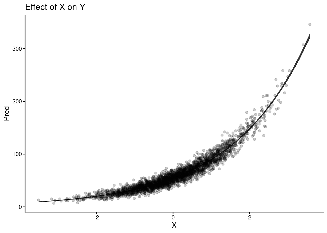
Extract predictions of Y ~ X

Here, I use a long-winded way to compute the predictions to show how it is done

Code

#create dataframe with values of X for which we want to predict Y
new_dat_Y_X <- tibble(X = seq(from = min(data$X), to = max(data$X), length.out = 30)) 

#predict Y but on the link scale (log) to calculate confidence intervals
pred_new_dat_Y_X <- predict(mY_X, newdata = new_dat_Y_X, type = "link", se.fit = TRUE)

#extract the inverse link function for the model (exponential in this case) 
ilink<- family(mY_X)$linkinv
# bind the dataframes with values of X and the predicted Y values
predictions_Y_X <- cbind(new_dat_Y_X,data.frame(pred_new_dat_Y_X)) %>%
  #calculate the confidence intervals on the log scale and exponentiate
  mutate(CI.up = ilink(fit + (1.96*se.fit)),
         CI.low = ilink(fit - (1.96*se.fit)),
         Pred=ilink(fit))

Plot

Code

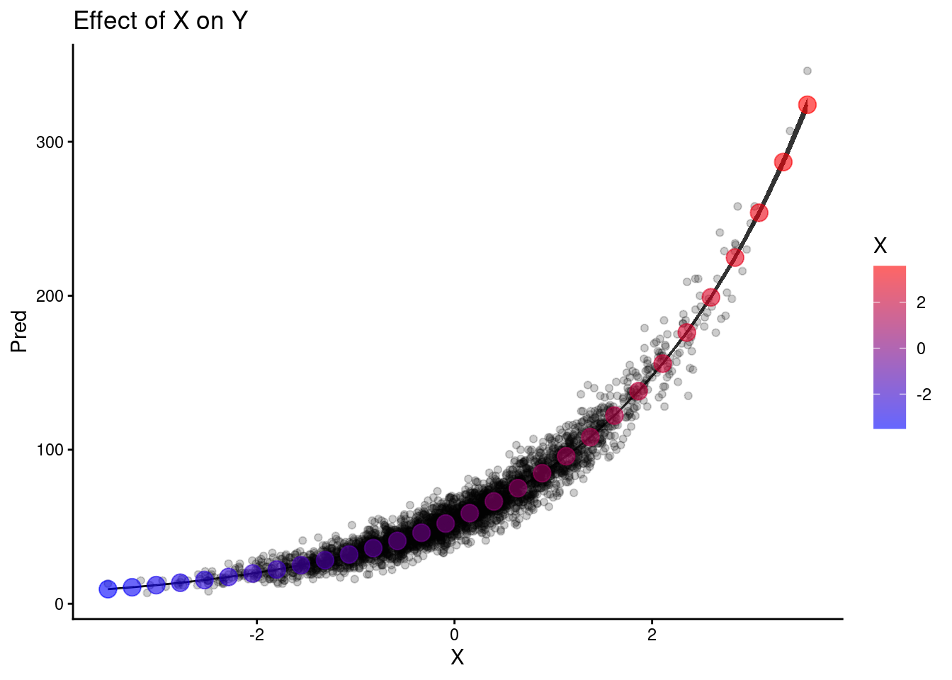
pY_X <- ggplot() +
  geom_line(data = predictions_Y_X, aes(y = Pred, x = X)) +
  geom_ribbon(data = predictions_Y_X, aes(ymin = CI.low, ymax = CI.up, x = X)) +
  geom_point(data = data, aes(x = X, y = Y), alpha = 0.2) +
  theme_classic() +
  labs(title = "Effect of X on Y")

pY_X

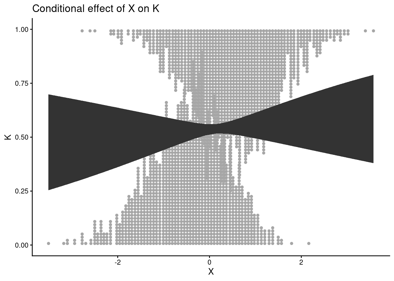
Now, the conditional (direct) effect of X on K

Code

new_dat_K_X <- tibble(X = seq(from = min(data$X), to = max(data$X), length.out = 30),
                      Y = mean(data$Y)) # set y to its mean to 

pred_new_dat_K_X <- predict(mK_XY, newdata = new_dat_K_X, type = "link", se.fit = TRUE)

ilink<- family(mK_XY)$linkinv
predictions_K_X <- cbind(new_dat_K_X,data.frame(pred_new_dat_K_X)) %>%
  mutate(CI.up = ilink(fit + (1.96*se.fit)),
         CI.low = ilink(fit - (1.96*se.fit)),
         Pred=ilink(fit))


pK_X <- ggplot() +
  stat_dots(data = data,
            aes(y = K,
                x = X,
                side = ifelse(K_1 == 0, "bottom", "top")),
            size = 2)+
  geom_line(data = predictions_K_X, aes(y = Pred, x = X)) +
  geom_ribbon(data = predictions_K_X, aes(ymin = CI.low, ymax = CI.up, x = X)) +
  
  theme_classic() +
  labs(title = "Conditional effect of X on K")

pK_X

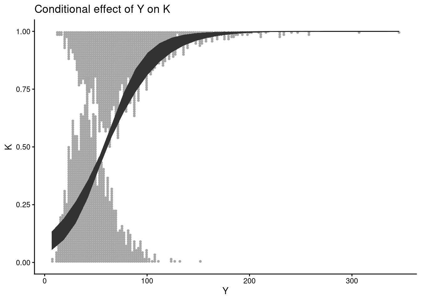
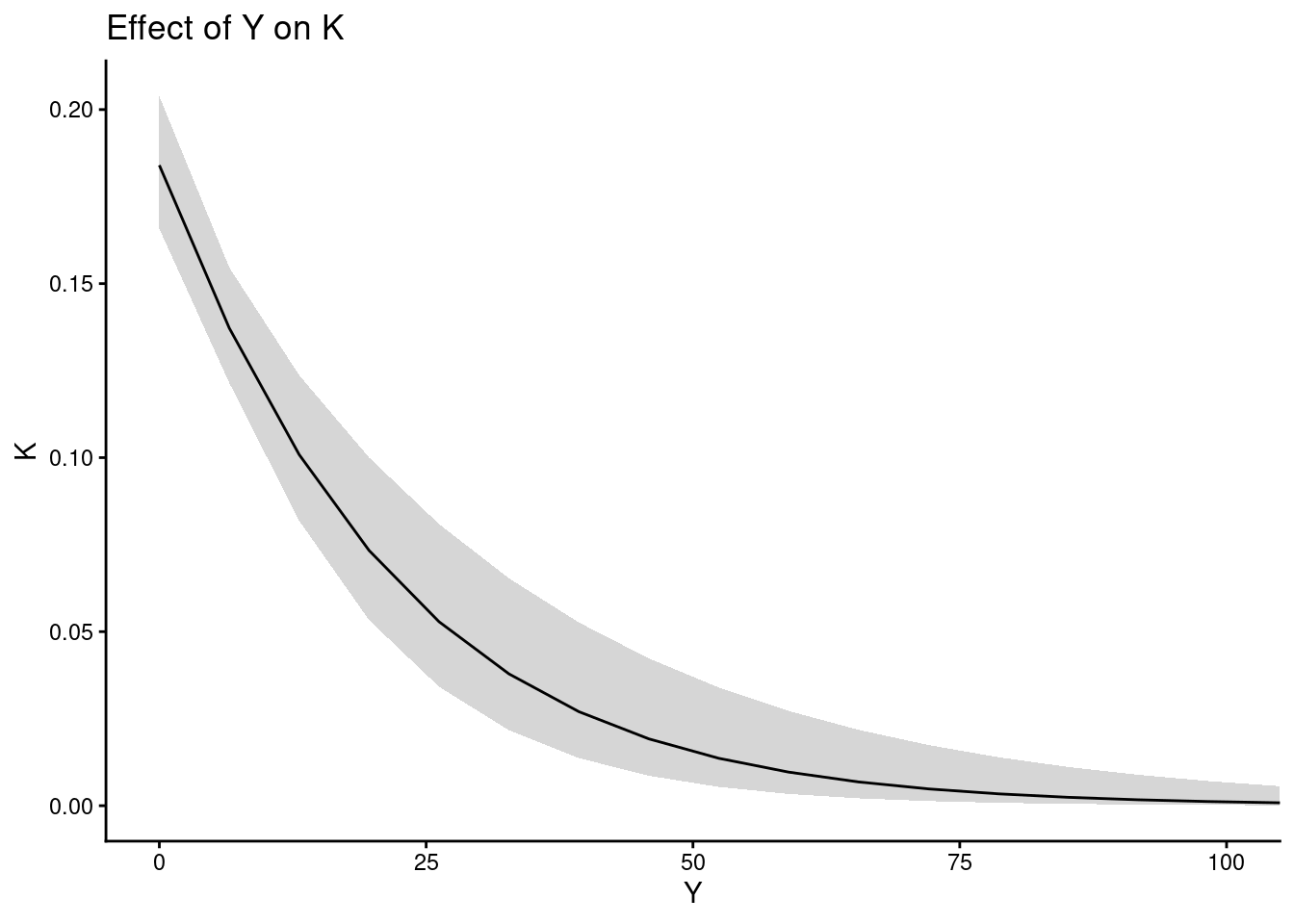
What about the conditional (direct) effect of Y on K ?

Code

new_dat_K_Y <- tibble(Y = seq(from = min(data$Y), to = max(data$Y), length.out = 30),
                      X = mean(data$X)) # set X to its mean

pred_new_dat_K_Y <- predict(mK_XY, newdata = new_dat_K_Y, type = "link", se.fit = TRUE)

ilink<- family(mK_XY)$linkinv
predictions_K_Y <- cbind(new_dat_K_Y,data.frame(pred_new_dat_K_Y)) %>%
  mutate(CI.up = ilink(fit + (1.96*se.fit)),
         CI.low = ilink(fit - (1.96*se.fit)),
         Pred=ilink(fit))

pK_Y <- ggplot() +
  stat_dots(data = data,
            aes(y = K,
                x = Y,
                side = ifelse(K_1 == 0, "bottom", "top")),
            size = 2)+
  geom_line(data = predictions_K_Y, aes(y = Pred, x = Y)) +
  geom_ribbon(data = predictions_K_Y, aes(ymin = CI.low, ymax = CI.up, x = Y)) +
  theme_classic() +
  labs(title = "Conditional effect of Y on K")

pK_Y

So this is the direct effect of Y on K. But, remember that Y is caused by X so it may be of interest to see how X affects K indirectly, through Y

Code

pY_X

The first step is to select values of Y that are predicted by X

Code

COLS <- alpha(colorRampPalette(c("blue","red"))(30),0.6)
pY_X + geom_point(data = predictions_Y_X, aes(y = Pred, x = X, color = X), size = 4) +scale_color_gradientn(colours = COLS)

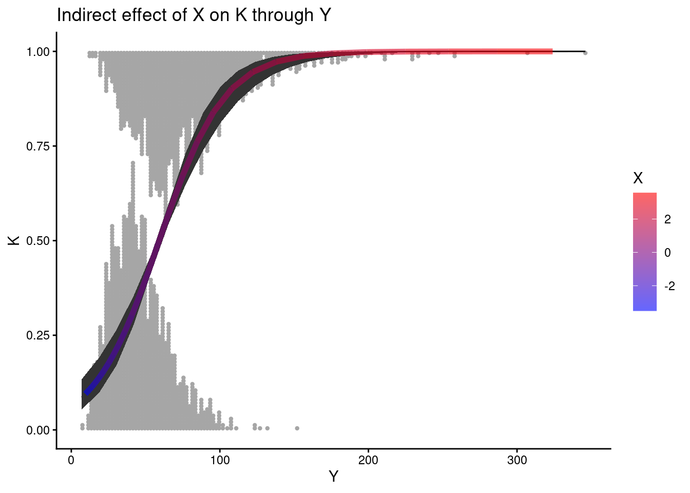
The next step is actually quite simple. We generate predictions for K as a function of the predictions of Y ~ X

new_dat_K_YX <- tibble(Y = predictions_Y_X$Pred, # predicted mean Y from X
                      X = mean(data$X)) # set X to its mean

Code

pred_new_dat_K_YX <- predict(mK_XY, newdata = new_dat_K_YX, type = "link", se.fit = TRUE)

ilink<- family(mK_XY)$linkinv
predictions_K_YX <- cbind(new_dat_K_YX,data.frame(pred_new_dat_K_YX)) %>%
  mutate(CI.up = ilink(fit + (1.96*se.fit)),
         CI.low = ilink(fit - (1.96*se.fit)),
         Pred=ilink(fit))

Now, we need the values of X that were associated with the predicted values of Y

Code

pred_K_YX <- select(predictions_K_YX, c(Y, Pred)) %>%
  left_join(predictions_Y_X %>% 
              select(X, Pred) %>% 
              rename(Y = Pred), 
            by = "Y")

pred_K_YX

Now, we simply superimpose both graphs of K ~ Y

Code

pK_Y

Code

pK_Y + geom_line(data = pred_K_YX, aes(x = Y, y = Pred, color = X), linewidth= 2) +
  labs(title = "Indirect effect of X on K through Y") + scale_color_gradientn(colours = COLS)

We could push this even further and look at indirect effects through a non-monotonous relationship

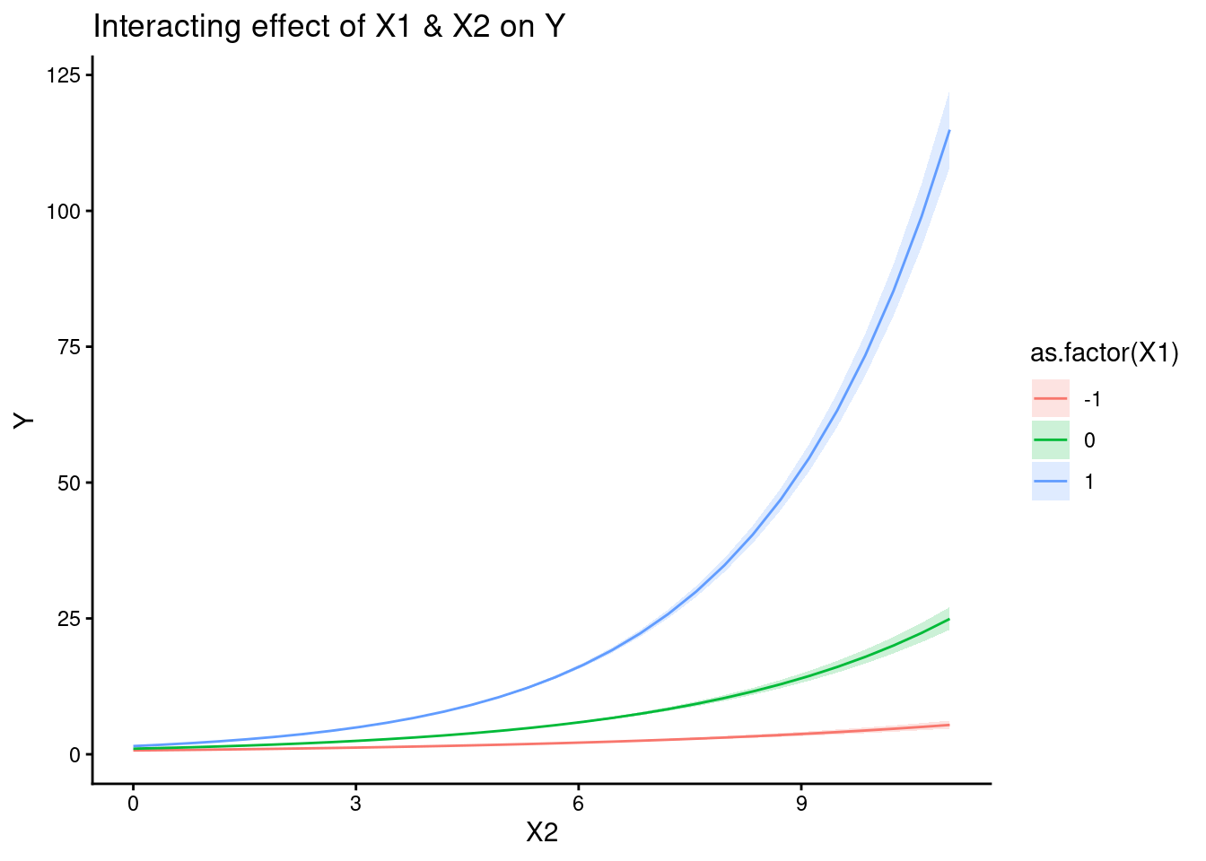
And what about interactions?

Simulate data

Code

n <- 3000
#interacting variables
X1 <- rnorm(n = n, mean = 0, sd = 1)
X2 <- rpois(n = n, lambda = 3)
#mediator
Y <- rpois(n = n, lambda = exp(0 + 0.4*X1 + 0.3*X2 + 0.1*X1*X2))
#outcome
K <- rbinom(n = n, size = 1, prob = plogis(-2 + 0.1*X1 + 0.2*X2 + 0.5*X1*X2 - 0.05*Y))

data <- tibble(
  X1 = X1,
  X2 = X2,
  Y = Y,
  K = K,
  K_1 = K - 1
)

head(data)

# A tibble: 6 × 5
      X1    X2     Y     K   K_1
   <dbl> <int> <int> <int> <dbl>
1  1.49      4    12     1     0
2  0.582     4     6     0    -1
3  1.30      1     3     0    -1
4 -2.01      1     0     0    -1
5  1.64      3     7     1     0
6  0.260     2     3     1     0

Models

Code

mY_X <- glmmTMB(Y ~  X1 + X2 + X1*X2, family = poisson, data = data)

mK_XY <- glmmTMB(K ~ X1 + X2 + X1*X2 + Y, family = binomial, data = data)

Predictions

Y ~ X

Code

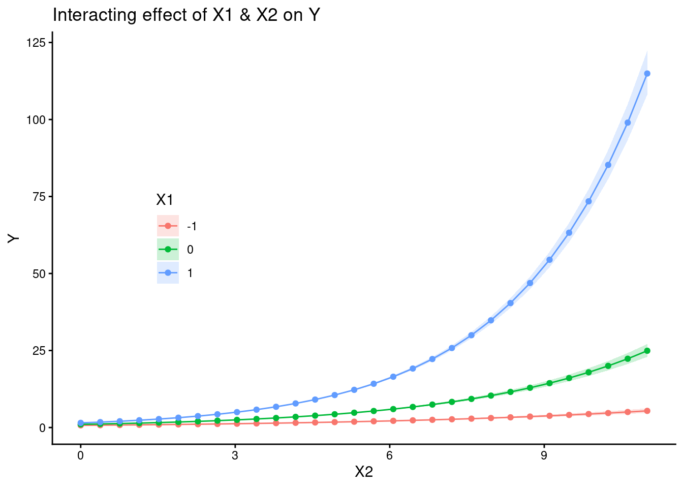
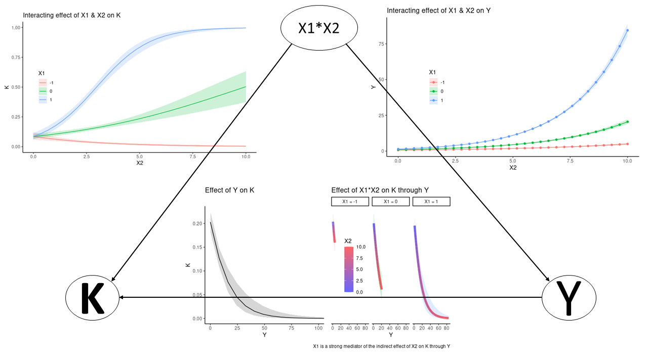
new_data_YX <- expand_grid(X1 = c(-1, 0, 1),
                           X2 = seq(from = min(data$X2), to = max(data$X2), length.out = 30))


pred_new_dat_Y_X <- predict(mY_X, newdata = new_data_YX, type = "link", se.fit = TRUE) # predict on link scale

ilink<- family(mY_X)$linkinv # extract inverse link (exponential in this case)

#calculate confidence intervals on link scale and back transform
predictions_Y_X <- cbind(new_data_YX,data.frame(pred_new_dat_Y_X)) %>%
  mutate(CI.up = ilink(fit + (1.96*se.fit)),
         CI.low = ilink(fit - (1.96*se.fit)),
         Pred=ilink(fit))

ggplot() +
  geom_ribbon(data = predictions_Y_X, aes(ymin = CI.low, ymax = CI.up, x = X2, fill = as.factor(X1)), alpha = 0.2) +
  geom_line(data = predictions_Y_X, aes(y = Pred, x = X2, color = as.factor(X1))) +
  labs(y = "Y",
       title = "Interacting effect of X1 & X2 on Y") +
  theme_classic()

K ~ X | Y

Code

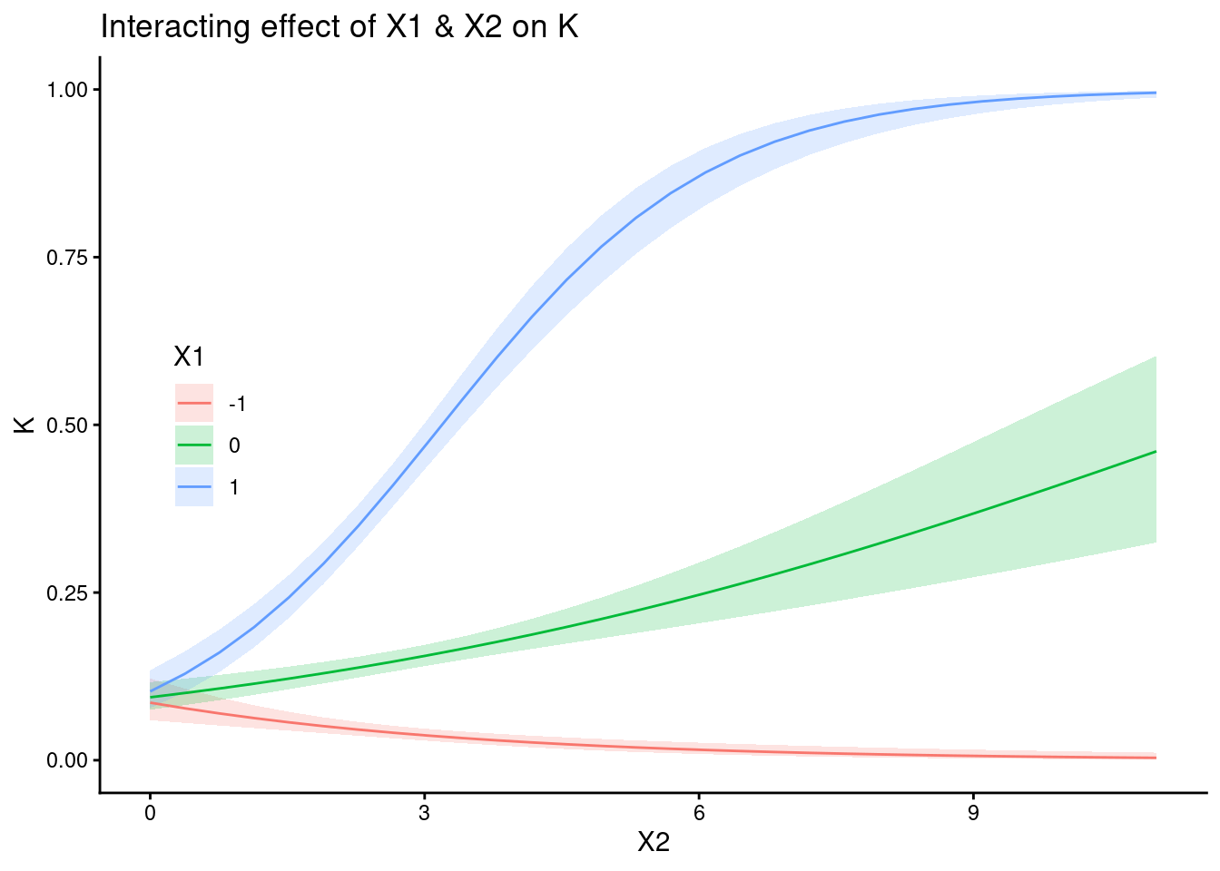
new_data_KX <- expand_grid(X1 = c(-1, 0, 1),
                           X2 = seq(from = min(data$X2), to = max(data$X2), length.out = 30),
                           Y = mean(data$Y))


pred_new_dat_K_X <- predict(mK_XY, newdata = new_data_KX, type = "link", se.fit = TRUE) # predict on link scale

ilink<- family(mK_XY)$linkinv # extract inverse link (inverse logit in this case)

#calculate confidence intervals on link scale and back transform
predictions_K_X <- cbind(new_data_KX,data.frame(pred_new_dat_K_X)) %>%
  mutate(CI.up = ilink(fit + (1.96*se.fit)),
         CI.low = ilink(fit - (1.96*se.fit)),
         Pred=ilink(fit))

pK_X <- ggplot() +
  geom_ribbon(data = predictions_K_X, aes(ymin = CI.low, ymax = CI.up, x = X2, fill = as.factor(X1)), alpha = 0.2) +
  geom_line(data = predictions_K_X, aes(y = Pred, x = X2, color = as.factor(X1)))+
  labs(y = "K",
       title = "Interacting effect of X1 & X2 on K",
       fill = "X1",
       color = "X1") +
  theme_classic()+theme(legend.position = c(0.1, 0.5))

pK_X

K ~ Y | X

Code

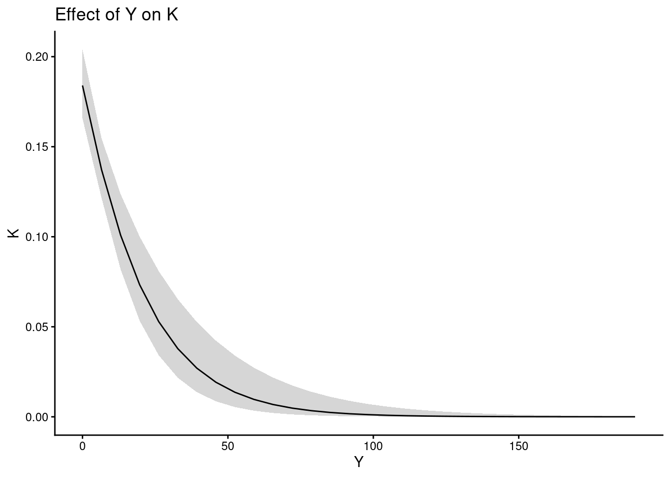
new_data_KY <- expand_grid(X1 = mean(data$X1),
                           X2 = mean(data$X2),
                           Y = seq(from = min(data$Y), to = max(data$Y), length.out = 30))


pred_new_dat_K_Y <- predict(mK_XY, newdata = new_data_KY, type = "link", se.fit = TRUE) # predict on link scale

ilink<- family(mK_XY)$linkinv # extract inverse link (inverse logit in this case)

#calculate confidence intervals on link scale and back transform
predictions_K_Y <- cbind(new_data_KY,data.frame(pred_new_dat_K_Y)) %>%
  mutate(CI.up = ilink(fit + (1.96*se.fit)),
         CI.low = ilink(fit - (1.96*se.fit)),
         Pred=ilink(fit))

ggplot() +
  geom_ribbon(data = predictions_K_Y, aes(ymin = CI.low, ymax = CI.up, x = Y), alpha = 0.2) +
  geom_line(data = predictions_K_Y, aes(y = Pred, x = Y))+
  labs(y = "K",
       title = "Effect of Y on K") +
  theme_classic()

K ~ E(Y|X)

Code

pY_X <- ggplot() +
  geom_ribbon(data = predictions_Y_X, aes(ymin = CI.low, ymax = CI.up, x = X2, fill = as.factor(X1)), alpha = 0.2) +
  geom_line(data = predictions_Y_X, aes(y = Pred, x = X2, color = as.factor(X1))) +
  geom_point(data = predictions_Y_X, aes(y = Pred, x = X2, color = as.factor(X1))) +
  labs(y = "Y",
       title = "Interacting effect of X1 & X2 on Y",
       color = "X1",
       fill = "X1") +
  theme_classic() +theme(legend.position = c(0.2, 0.5))

pY_X

need to predict K for the different predicted values of Y ~ X

Code

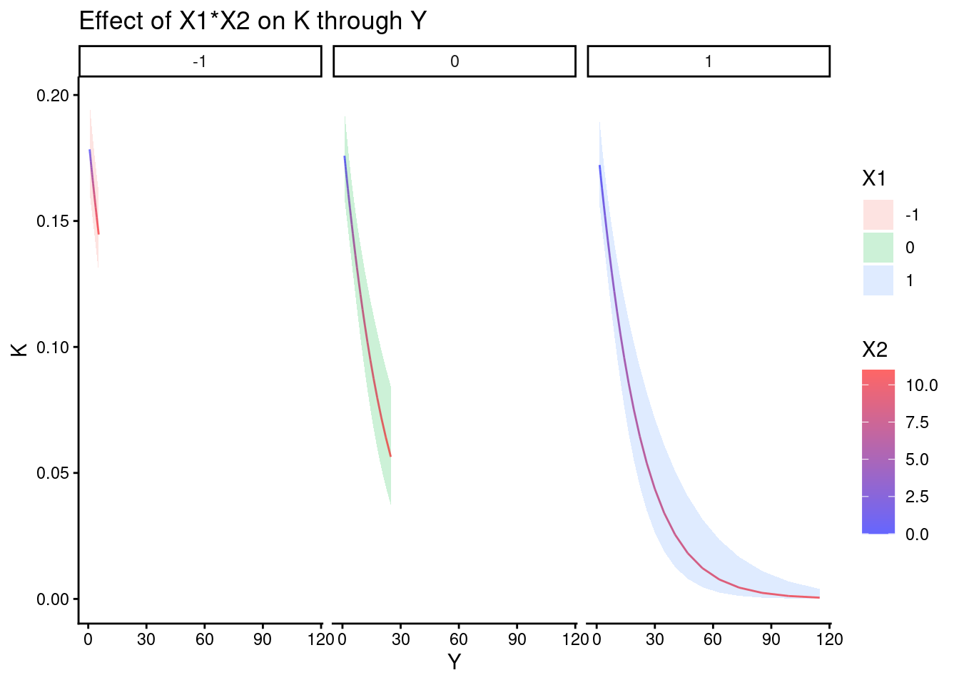
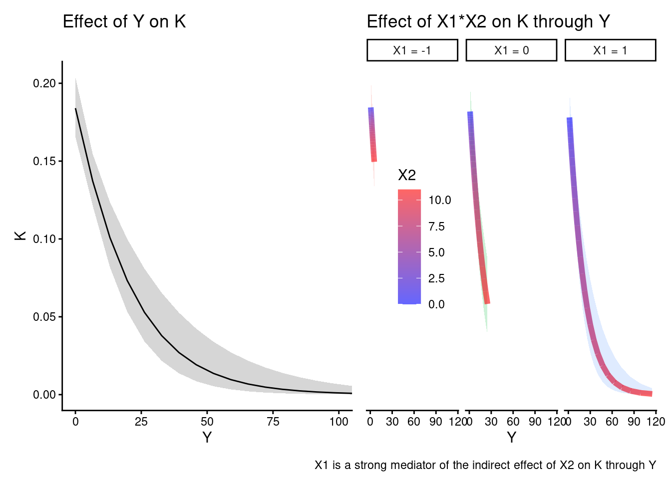
new_data_KYX <- tibble(
  Y = predictions_Y_X$Pred,
  X1 = mean(data$X1),
  X2 = mean(data$X2)
)

pred_new_dat_K_YX <- predict(mK_XY, newdata = new_data_KYX, type = "link", se.fit = TRUE) # predict on link scale

ilink<- family(mK_XY)$linkinv # extract inverse link (inverse logit in this case)

#calculate confidence intervals on link scale and back transform
predictions_K_YX <- cbind(new_data_KYX,data.frame(pred_new_dat_K_YX)) %>%
  mutate(CI.up = ilink(fit + (1.96*se.fit)),
         CI.low = ilink(fit - (1.96*se.fit)),
         Pred=ilink(fit)) %>%
  select(-c(X1, X2)) %>% #remove X1 and X2 that are set to their means as we don't need them
  mutate(X1 = predictions_Y_X$X1, 
         X2 = predictions_Y_X$X2)  # add the values of X1 and X2 that were used to predict Y
  
COLS <- alpha(colorRampPalette(c("blue","red"))(30),0.6)
ggplot() +
  geom_ribbon(data = predictions_K_YX, aes(ymin = CI.low, ymax = CI.up, x = Y, fill = as.factor(X1)), alpha = 0.2) +
  geom_line(data = predictions_K_YX, aes(y = Pred, x = Y,  color = X2))+
  scale_color_gradientn(colours = COLS)+
  labs(y = "K",
       title = "Effect of X1*X2 on K through Y",
       fill = "X1") +
  theme_classic() +
  facet_wrap(~as.factor(X1))

Make it “pretty”

Code

facet_labels_X1 <- as_labeller(
  c(
    `-1` = "X1 = -1",
    `0` = "X1 = 0",
    `1` = "X1 = 1"
  ))
pK_XY <- ggplot() +
  geom_ribbon(data = predictions_K_YX, aes(ymin = CI.low, ymax = CI.up, x = Y, fill = as.factor(X1)), alpha = 0.2) +
  geom_line(data = predictions_K_YX, aes(y = Pred, x = Y,  color = X2), linewidth = 2)+
  scale_color_gradientn(colours = COLS)+
  labs(
       title = "Effect of X1*X2 on K through Y") +
  guides(fill = "none") +
  theme_classic() +
  facet_wrap(~as.factor(X1), labeller = facet_labels_X1)+
  theme(legend.position = c(0.2, 0.5),
        axis.line.y = element_blank(),
        axis.text.y = element_blank(),
        axis.ticks.y = element_blank(),
        axis.title.y = element_blank())

pK_XY

pK_Y

Code

pK_Y <- ggplot() +
  geom_ribbon(data = predictions_K_Y, aes(ymin = CI.low, ymax = CI.up, x = Y), alpha = 0.2) +
  geom_line(data = predictions_K_Y, aes(y = Pred, x = Y))+
  labs(y = "K",
       title = "Effect of Y on K") +
  coord_cartesian(xlim = c(0, 100)) +
  theme_classic()

pK_Y

patchwork

Code

patch_K_Y <- pK_Y + pK_XY + plot_annotation(caption = "X1 is a strong mediator of the indirect effect of X2 on K through Y")

patch_K_Y

Bring it all together

Citation

BibTeX citation:

@online{bush-beaupré2023,
  author = {Bush-Beaupré, Allen},
  title = {Visualizing Indirect Effects},
  date = {2023-10-31},
  url = {https://abushbeaupre.github.io/posts/indirect_effects/},
  langid = {en}
}

For attribution, please cite this work as:

Bush-Beaupré, Allen. 2023. “Visualizing Indirect Effects.” October 31, 2023. https://abushbeaupre.github.io/posts/indirect_effects/.