Introduction

In this third part of my tutorial series on statistical interactions, we are going to push further on our understanding and reporting of interactions. Since we are going beyond the realm of linear models by exploring generalized linear models (GLMs) and their variants, I am assuming here that the reader has a basic understanding of how GLMs work especially concerning their use of link functions.

I typically write up these tutorials based on bits and pieces of information I have gathered here and there but I will (in part) address topics covered by Spake et al. (2023) https://onlinelibrary.wiley.com/doi/full/10.1111/brv.12939 while giving examples of tools that can be used to report interaction effects on the additive and multiplicative scale.

The case studies in this tutorial will focus on species occurence and abundance. We will first look at habitat suitability for a given species to occur in a given location. Second, we will explore factors that affect their abundance when they are present. Third, we will incorporate both these processes in a single model and learn how to extract as much information as possible from these types of analyses.

Setup

First, we load the relevant packages and set up our ggplot2 theme for the rest of the document.

library(tidyverse)       # Data manipulation and plotting
library(tidylog)         # Print a log of data manipulations done with tidyverse
library(glmmTMB)         # Generalized linear (mixed) models
library(marginaleffects) # Compute marginal/condition effects
library(patchwork)       # Combine multiple plots
library(distributional)  # Simulate distributions
library(ggdist)          # Plot nice distributions
library(GGally)

# Set ggplot2 theme
black_theme <- theme(
  axis.line = element_line(linewidth = 2, lineend = "round", color = "white"),
  panel.grid = element_blank(),
  panel.background = element_rect(fill = "black", color = NA),
  axis.ticks = element_blank(),
  axis.text = element_text(size = 21, face = "bold", color = "white"),
  axis.title = element_text(size = 21, face = "bold", color = "white"),
  plot.title = element_text(size = 25, face = "bold", color = "white"),
  plot.background = element_rect(fill = "black", color = NA),
  legend.background = element_rect(fill = "black", color = NA),
  legend.text = element_text(size = 21, color = "white"),
  legend.title = element_text(size = 21, face = "bold", color = "white"),
  legend.position = "bottom"
)

theme_set(black_theme)

# Set global default for geom_point shape
update_geom_defaults("point", list(shape = 1, size = 3, alpha = 0.8))

# silence marginaleffects warnings about glmmTMB
options(marginaleffects_safe = FALSE)

set.seed(333)

Case Study 1: Species occurence

In this first case study, we are interested in species occurence in different habitats. Specifically, we want evaluate the the interacting effects of habitat composition and environmental variables on the probability of occurence in a given patch.

https://ben18785.shinyapps.io/distribution-zoo/

n_plots <- 200

tree_cover <- dist_mixture(dist_beta(4, 0.8), dist_beta(0.8, 4), weights = c(0.5, 0.5))

avg_yearly_rain <- dist_gamma(shape = 3, rate = 0.7)

avg_yearly_temp <- dist_normal(mu = 20, sd = 10)

occurence_intercept <- plogis(-3)

occurence_tree_effect <- 0.45

occurence_rain_effect <- 0.01

occurence_temp_effect <- 0.01

tibble(
  tree = generate(tree_cover, n_plots),
  rain = generate(avg_yearly_rain, n_plots),
  temp = generate(avg_yearly_temp, n_plots)
) |> 
  unnest(everything()) |>
  mutate(occurence = rbinom(n_plots, size = 1, 
                     prob = occurence_intercept +
                            occurence_tree_effect * tree +
                            occurence_rain_effect * rain +
                            occurence_temp_effect * temp
                            ))-> occ_data

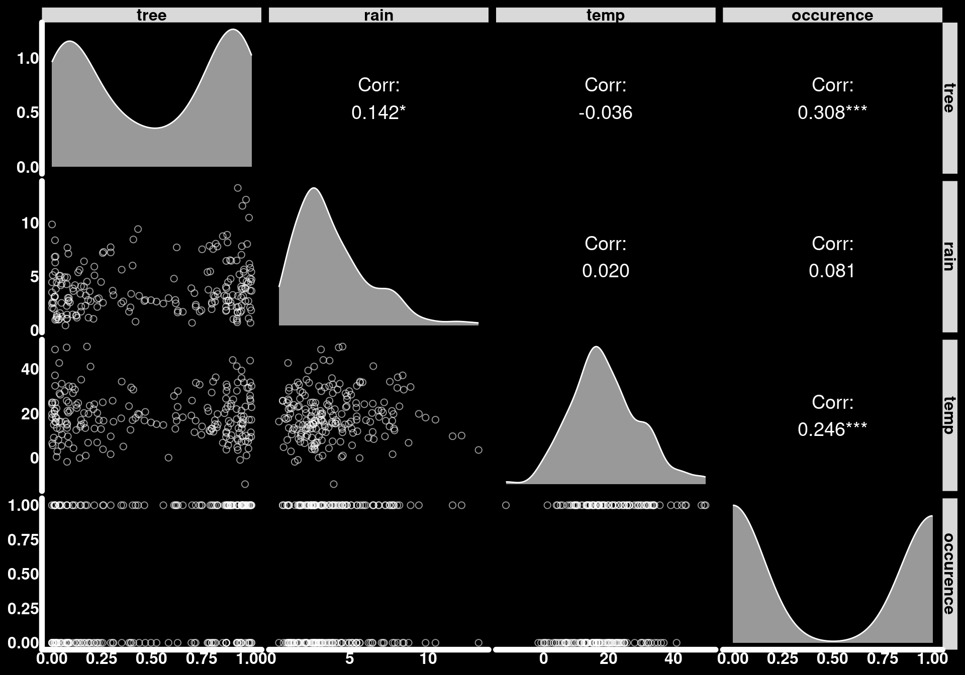
mutate: new variable 'occurence' (integer) with 2 unique values and 0% NA

ggpairs(
  occ_data,
  diag  = list(continuous = wrap("densityDiag", fill = "white", alpha = 0.6, color = "white")),
  lower = list(continuous = wrap("points", color = "white", alpha = 0.6, size = 2, shape = 1)),
  upper = list(continuous = wrap("cor", color = "white", size = 5))
) +
  theme(
    strip.text = element_text(color = "black", face = "bold", size = 12),
    axis.text = element_text(color = "white", face = "bold", size = 12)
  )

Some people might want to dichotomize tree cover

occ_data |>
  mutate(tree_cat = as.factor(ifelse(tree > 0.5, "high", "low"))) -> occ_data

mutate: new variable 'tree_cat' (factor) with 2 unique values and 0% NA

Implicit interactions

scale_x <- function(x){
  x - mean(x) / sd(x)
}

occ_data |>
  mutate(scl_tree = scale_x(tree),
         scl_rain = scale_x(rain),
         scl_temp = scale_x(temp)) -> occ_data

mutate: new variable 'scl_tree' (double) with 200 unique values and 0% NA
        new variable 'scl_rain' (double) with 200 unique values and 0% NA
        new variable 'scl_temp' (double) with 200 unique values and 0% NA

mod_1 <- glmmTMB(occurence ~ tree + rain + temp, family = binomial(link = "logit"), data = occ_data)

summary(mod_1)

 Family: binomial  ( logit )
Formula:          occurence ~ tree + rain + temp
Data: occ_data

      AIC       BIC    logLik -2*log(L)  df.resid 
    250.0     263.2    -121.0     242.0       196 


Conditional model:
            Estimate Std. Error z value Pr(>|z|)    
(Intercept) -2.27069    0.49227  -4.613 3.98e-06 ***
tree         1.87063    0.42528   4.399 1.09e-05 ***
rain         0.03176    0.06486   0.490 0.624346    
temp         0.05805    0.01579   3.675 0.000238 ***
---
Signif. codes:  0 '***' 0.001 '**' 0.01 '*' 0.05 '.' 0.1 ' ' 1

slopes(mod_1, variables = "tree", newdata = datagrid(temp = mean(occ_data$temp), rain = mean(occ_data$rain)))


 temp rain Estimate Std. Error   z Pr(>|z|)    S 2.5 % 97.5 %
   19  3.9    0.467      0.106 4.4   <0.001 16.5 0.259  0.675

Term: tree
Type: response
Comparison: dY/dX

avg_slopes(mod_1, variables = "rain")


 Estimate Std. Error     z Pr(>|z|)   S   2.5 % 97.5 %
  0.00663     0.0135 0.491    0.624 0.7 -0.0199 0.0331

Term: rain
Type: response
Comparison: dY/dX

avg_slopes(mod_1, variables = "temp")


 Estimate Std. Error   z Pr(>|z|)    S   2.5 % 97.5 %
   0.0121    0.00288 4.2   <0.001 15.2 0.00647 0.0178

Term: temp
Type: response
Comparison: dY/dX

slopes(mod_1, variables = "tree", newdata = datagrid(temp = fivenum, rain = fivenum)) -> t

ggplot(t) + geom_pointrange(aes(x = estimate, xmin = conf.low, xmax = conf.high, y = 1), color = "white") +
  geom_vline(xintercept = occurence_tree_effect, color = "white", alpha = .8) +
  facet_grid(rain ~ temp)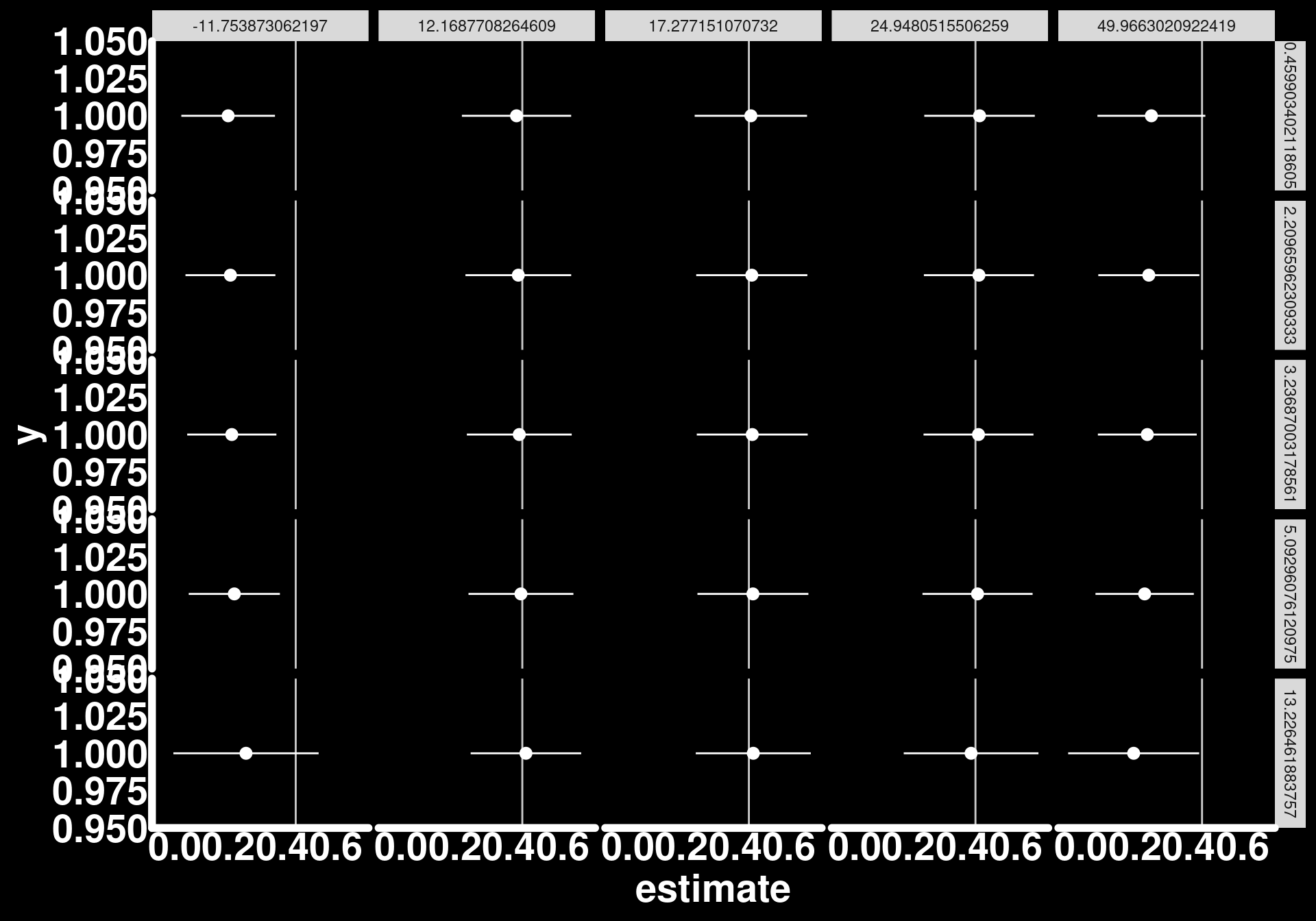

predictions(mod_1, variables = "tree", newdata = datagrid(temp = fivenum, rain = fivenum)) -> pred_tree1

ggplot(pred_tree1) +
  geom_ribbon(aes(x = tree, ymin = conf.low, ymax = conf.high), fill = "white", alpha = 0.2) +
  geom_line(aes(x = tree, y = estimate), color = "white") +
  facet_grid(rain ~ temp)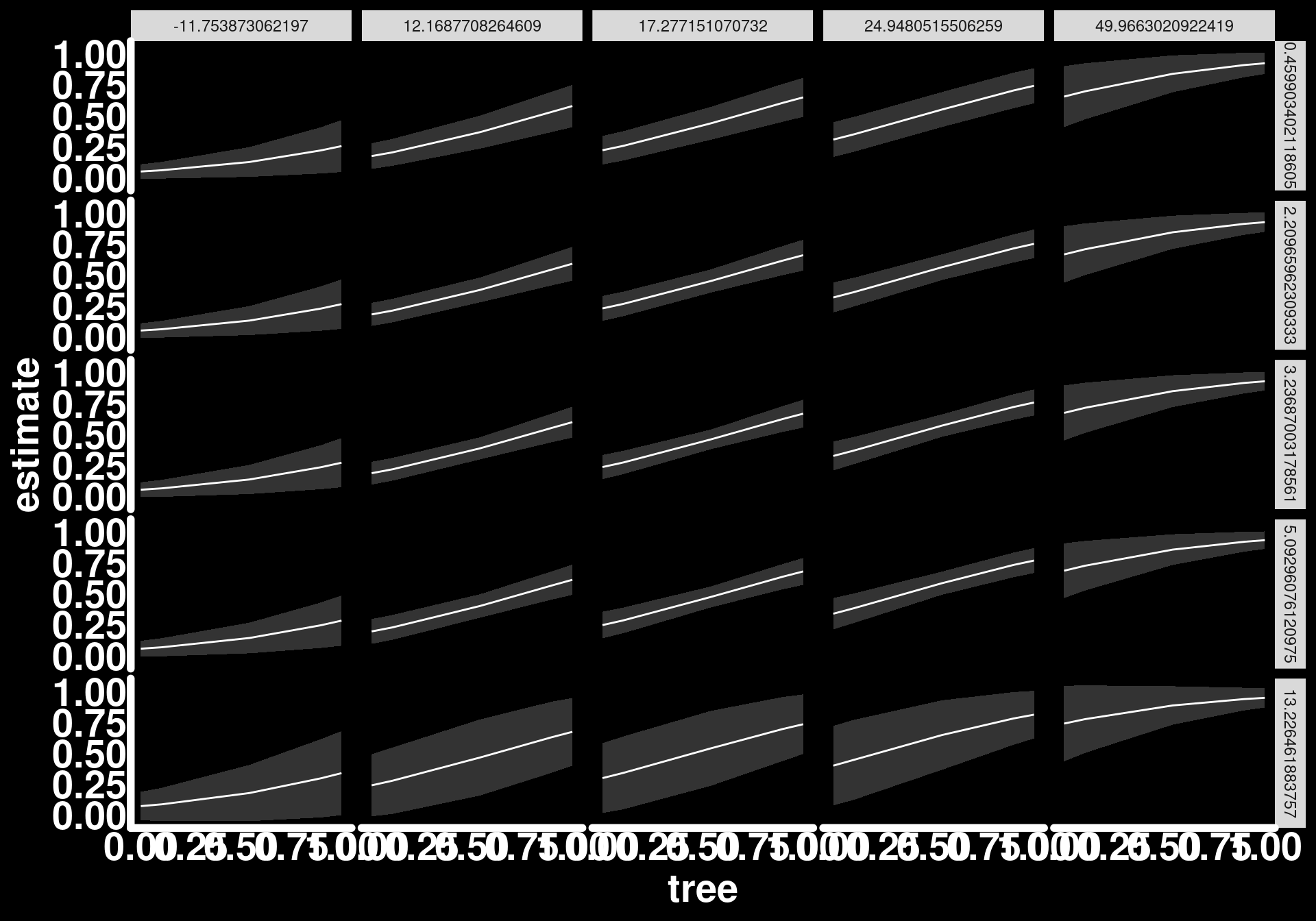

avg_slopes(mod_1, variables = "tree")


 Estimate Std. Error    z Pr(>|z|)    S 2.5 % 97.5 %
    0.391     0.0715 5.46   <0.001 24.3  0.25  0.531

Term: tree
Type: response
Comparison: dY/dX

slopes(mod_1, variables = "tree", newdata = datagrid(temp = 0, rain = 0))


 temp rain Estimate Std. Error    z Pr(>|z|)   S 2.5 % 97.5 %
    0    0    0.312     0.0986 3.16  0.00156 9.3 0.119  0.505

Term: tree
Type: response
Comparison: dY/dX

slopes(mod_1, variables = "tree", newdata = datagrid(temp = mean(occ_data$temp), rain = mean(occ_data$rain)))


 temp rain Estimate Std. Error   z Pr(>|z|)    S 2.5 % 97.5 %
   19  3.9    0.467      0.106 4.4   <0.001 16.5 0.259  0.675

Term: tree
Type: response
Comparison: dY/dX

avg_slopes(mod_1, variables = "rain")


 Estimate Std. Error     z Pr(>|z|)   S   2.5 % 97.5 %
  0.00663     0.0135 0.491    0.624 0.7 -0.0199 0.0331

Term: rain
Type: response
Comparison: dY/dX

slopes(mod_1, variables = "rain", newdata = datagrid(temp = 0, tree = 0))


 temp tree Estimate Std. Error     z Pr(>|z|)   S    2.5 % 97.5 %
    0    0  0.00298    0.00622 0.478    0.632 0.7 -0.00921 0.0152

Term: rain
Type: response
Comparison: dY/dX

slopes(mod_1, variables = "rain", newdata = datagrid(temp = mean(occ_data$temp), tree = mean(occ_data$tree)))


 temp tree Estimate Std. Error    z Pr(>|z|)   S   2.5 % 97.5 %
   19 0.51  0.00792     0.0162 0.49    0.624 0.7 -0.0238 0.0396

Term: rain
Type: response
Comparison: dY/dX

avg_slopes(mod_1, variables = "temp")


 Estimate Std. Error   z Pr(>|z|)    S   2.5 % 97.5 %
   0.0121    0.00288 4.2   <0.001 15.2 0.00647 0.0178

Term: temp
Type: response
Comparison: dY/dX