Audience: graduate students and researchers in ecology who fit GL(M)Ms and want to interpret interaction terms correctly.
Format: short lecture blocks, live-coded examples, and practice exercises (look for the 🧪 slides).
Learning objectives
By the end of this workshop you should be able to:
Explain what an interaction term means for a categorical × numerical model and for a numerical × numerical model
Distinguish conditional effects from marginal effects, and choose the right one for a research question
Recognize Simpson’s Paradox and sampling bias as threats to naive interpretation
Learning objectives (continued)
Use marginaleffects (predictions(), slopes(), avg_predictions(), avg_slopes(), hypotheses()) to extract and test the quantities you actually care about
Visualize interaction effects (slope-by-moderator plots, five-number-summary predictions, response surfaces) and know their trade-offs
Setup
library(tidyverse) # Data manipulation and plottinglibrary(glmmTMB) # Generalized linear (mixed) modelslibrary(marginaleffects) # Compute marginal/conditional effectslibrary(patchwork) # Combine multiple plotslibrary(GGally) # Pairwise plots# Set ggplot2 themeblack_theme <-theme(axis.line =element_line(linewidth =2, lineend ="round", color ="white"),panel.grid =element_blank(),panel.background =element_rect(fill ="black", color =NA),axis.ticks =element_blank(),axis.text =element_text(size =21, face ="bold", color ="white"),axis.title =element_text(size =21, face ="bold", color ="white"),plot.title =element_text(size =25, face ="bold", color ="white"),plot.background =element_rect(fill ="black", color =NA),legend.background =element_rect(fill ="black", color =NA),legend.text =element_text(size =21, color ="white"),legend.title =element_text(size =21, face ="bold", color ="white"),legend.position ="bottom")theme_set(black_theme)# Set global default for geom_point shapeupdate_geom_defaults("point", list(shape =1, size =3, alpha =0.8))# silence marginaleffects warnings about glmmTMBoptions(marginaleffects_safe =FALSE)set.seed(4127)
\(\beta_3\) is the interaction coefficient. When \(\beta_3 \neq 0\), the effect of \(X_1\) on \(Y\)depends on the value of\(X_2\).
For a categorical \(X_2\) (e.g., sex) and continuous \(X_1\) (e.g., snow depth): the interaction means the slope of the continuous predictor differs between categories.
Conditional vs. marginal effects
Conditional effects: the effect of a predictor at specific values of other predictors (e.g., the slope of snow depth for males)
Marginal effects: the effect averaged across the distribution of other predictors (e.g., the average slope of snow depth across the whole population)
Both are legitimate; they answer different questions. Interactions are exactly where the distinction starts to matter.
Case study: Bighorn sheep
Ram Mountain, Alberta. Question: how does winter snow depth relate to spring mass in Bighorn sheep, and does it differ by sex? Males and females segregate in winter — females use lower, less snowy habitat.
Built-in features: different intercepts, different slopes, and different snow-depth distributions by sex.
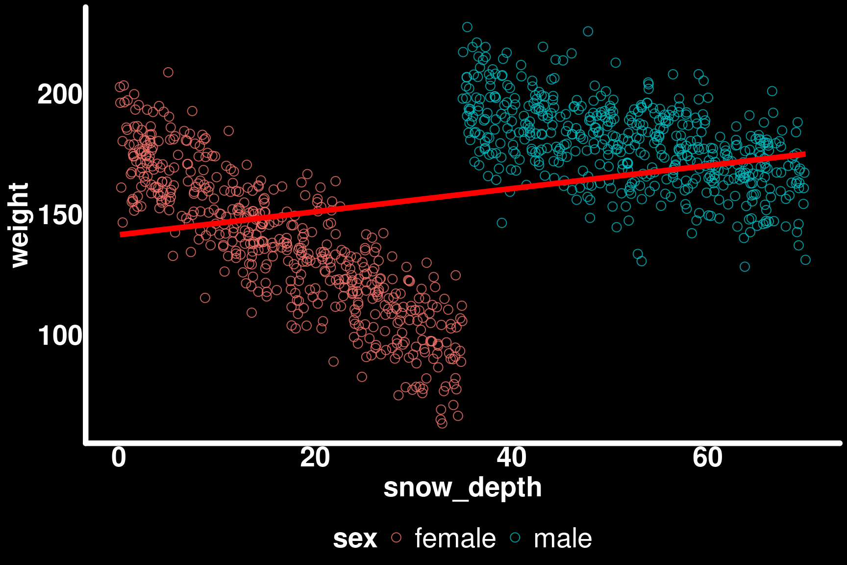
Simpson’s Paradox
Code
ggplot(bighorn_population, aes(x = snow_depth, y = weight)) +geom_point(aes(color = sex)) +geom_smooth(method ="lm", se =FALSE, color ="red", linewidth =2)
Ignoring sex hides the true within-sex trends.
Pooled: snow depth looks positively associated with weight — even though both sexes lose weight with more snow.
Why? Sex is a confounder
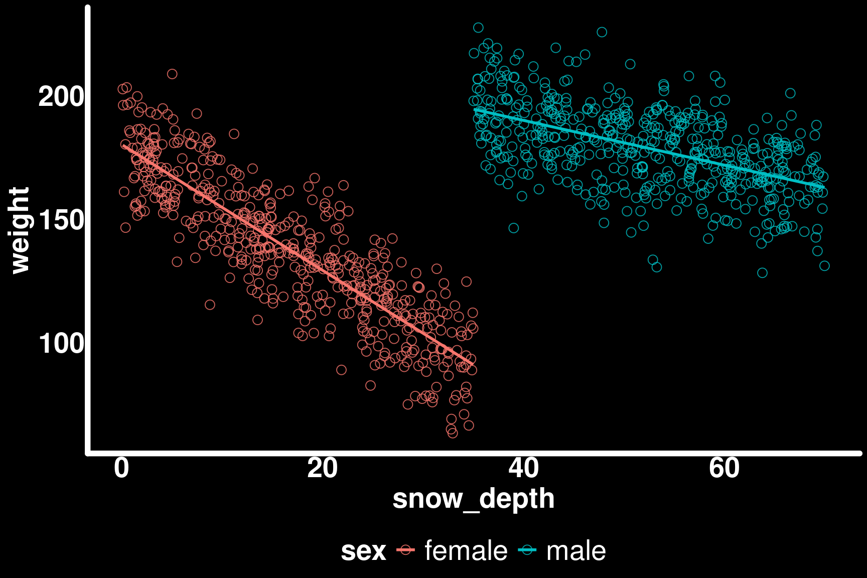
Within each sex: more snow → lower weight (true negative relationship)
Between sexes: males see more snow and are heavier (confounded)
Pooled data compares heavy, high-snow males to light, low-snow females → spurious positive trend
Within-sex trends
Code
ggplot(bighorn_population, aes(x = snow_depth, y = weight, color = sex)) +geom_point() +geom_smooth(method ="lm", se =FALSE)
Within-sex trends are negative, as expected.
🧪 Exercise 1
Using bighorn_population:
Fit weight ~ sex * snow_depth with glmmTMB(). Call it mod_mass_true.
From the summary, identify which coefficient represents the male slope of snow depth. (Hint: it’s not printed directly — you have to add two rows together.)
In one sentence, explain why a naive weight ~ snow_depth model (ignoring sex) would mislead a manager trying to understand the effect of a harsh winter.
(~5 minutes — discuss with a neighbor)
Sampling from the population
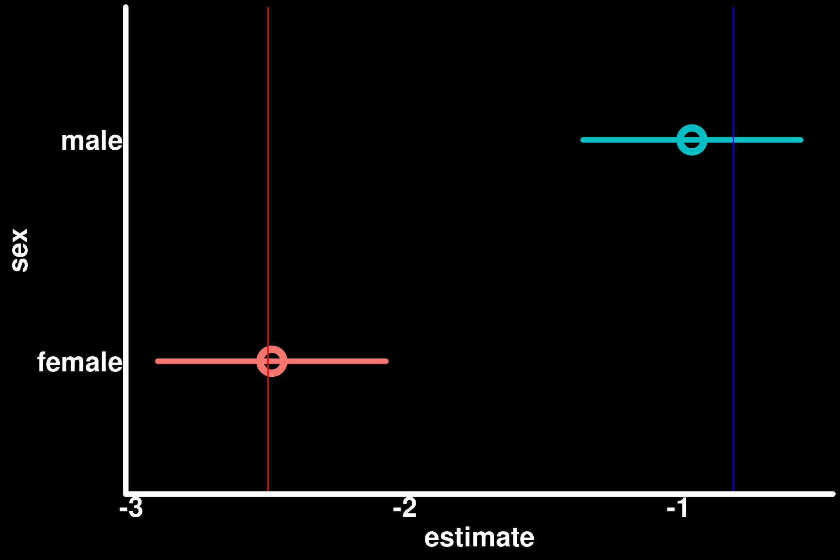
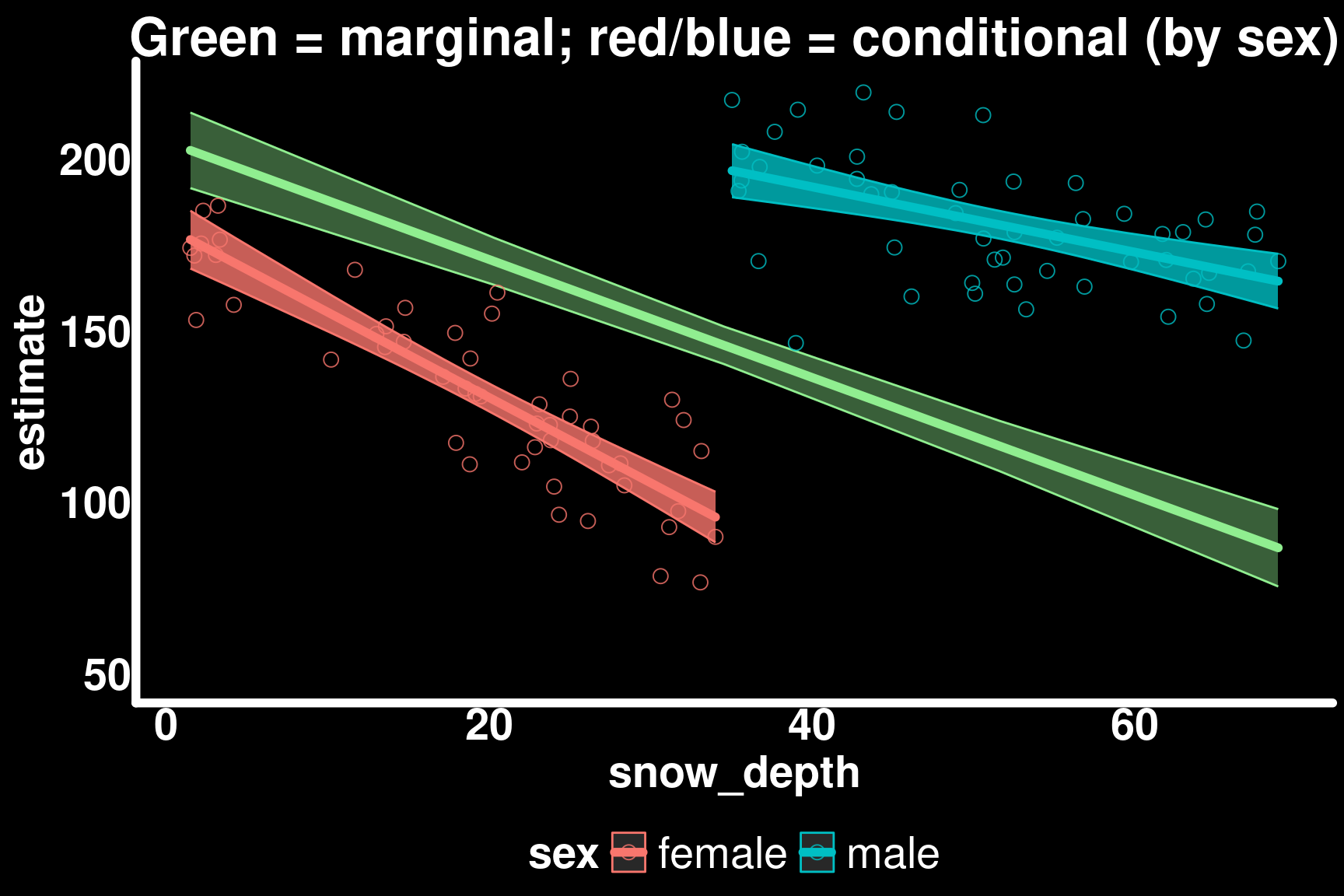
In practice we can’t measure everyone. Two sampling scenarios:
Conditional (by-sex) slopes stay close to truth. But the marginal slope is biased toward the overrepresented, weaker-effect sex (males).
Correcting for known sampling bias
If we know the true population sex ratio (50:50), we can average over a balancednewdata grid instead of our biased sample.
Key principle: model coefficients capture conditional relationships from your sample; marginal effects can target any population composition via newdata.
Compute avg_slopes()without correcting for sampling bias, and again with the balanced newdata_balanced grid.
Which one is closer to the true average slope, mean(c(male_loss, female_loss))?
Suppose instead you didn’t know the true sex ratio in the population — what additional data would you need to collect to justify a correction like this?
(~7 minutes — try it in your own script, then we’ll compare answers)
Part 1 takeaways
Interactions → conditional effects that depend on other variables
Simpson’s Paradox is a real risk when pooling across confounded groups
Marginal ≠ conditional; both are valid but answer different questions
Raw model coefficients rarely equal your research quantity of interest — use marginaleffects
Marginal effects inherit your sample’s covariate distribution unless you override it with newdata
The slope of \(X_1\) is now itself a linear function of\(X_2\): it equals \(\beta_1 + \beta_3 X_2\). Symmetrically, the slope of \(X_2\) is \(\beta_2 + \beta_3 X_1\).
\(\beta_1\) alone is only the slope of \(X_1\) when \(X_2 = 0\) — meaningful only if zero is a meaningful value of \(X_2\). This motivates centering.
Case study: petal length
Simulated flowers; petal length as a function of temperature and rain, with an interaction.
Predictors are mean-centered: the intercept becomes the predicted response at average conditions rather than at (biologically meaningless) zero temperature/rain.
Every term has a small p-value — but what do these numbers mean for our research question? Time to unpack them.
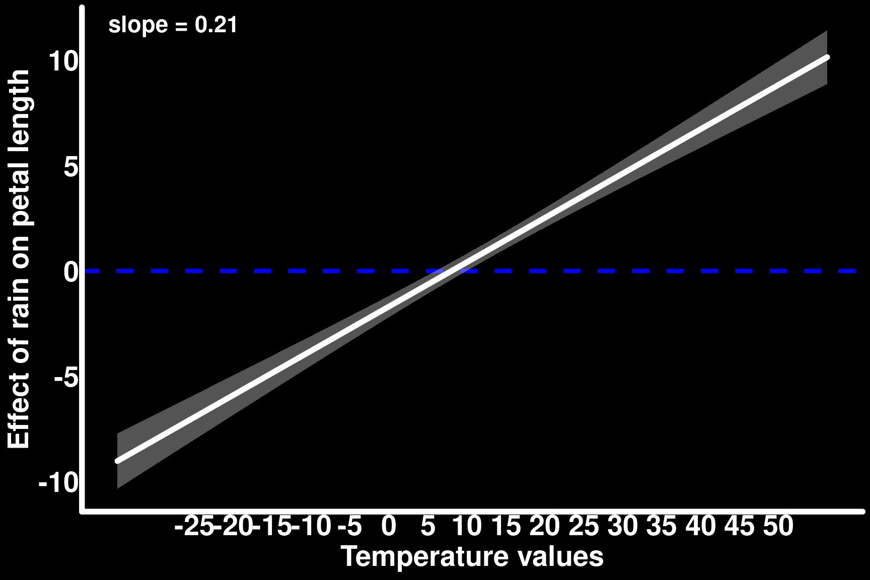
Slope of one predictor at a single value of the other
# Effect of temperature when rain_centered = 0 (i.e., average rain)slopes(mod_flower_1, newdata =datagrid(rain_centered =0),variables ="temp_centered")
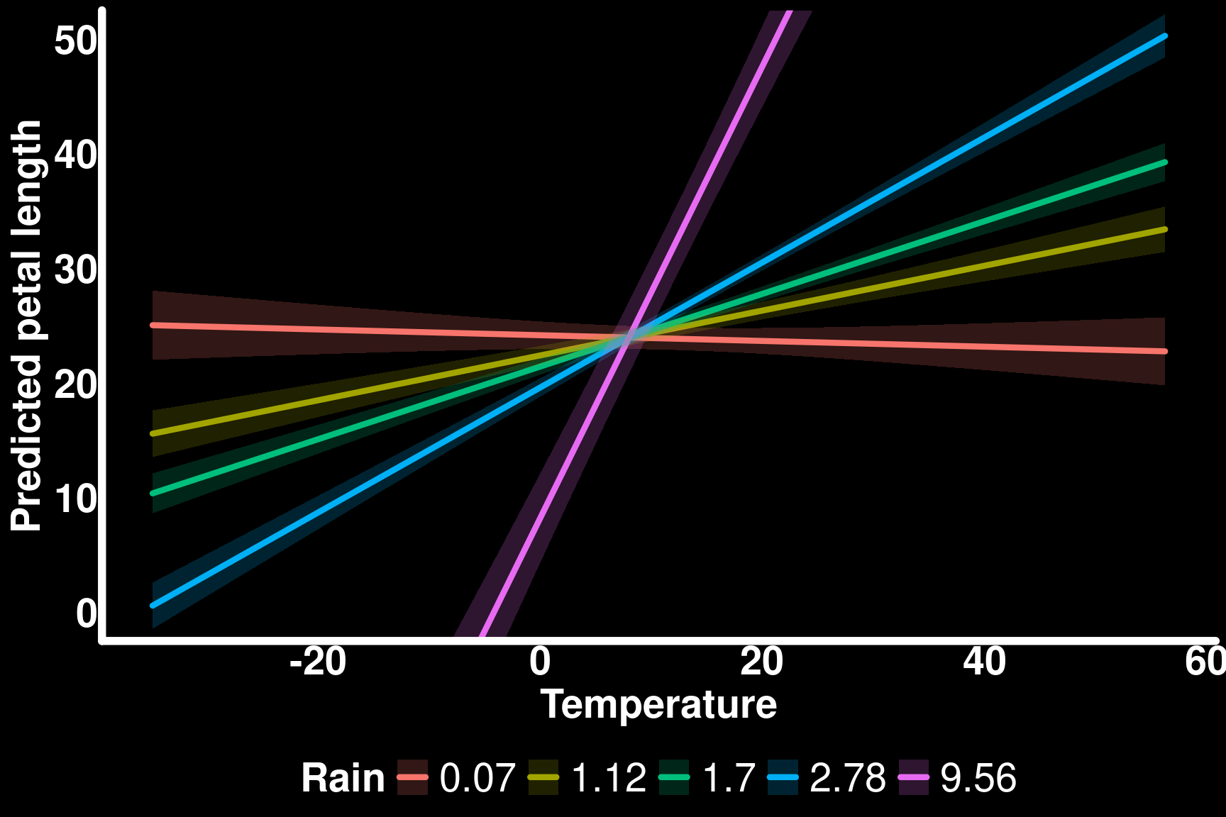
predictions(mod_flower_1,newdata =datagrid(temp_centered =seq(min(flower_measurements_1$temp_centered),max(flower_measurements_1$temp_centered), length.out =30),rain_centered = fivenum )) |>as_tibble() |>mutate(rain =round(rain_centered +mean(rain), 2)) |>ggplot() +geom_line(aes(y = estimate, x = temp_centered +mean(temperature), color =as.factor(rain)),lineend ="round", linewidth =1.5) +geom_ribbon(aes(ymin = conf.low, ymax = conf.high,x = temp_centered +mean(temperature), fill =as.factor(rain)), alpha =0.2) +labs(y ="Predicted petal length", x ="Temperature", color ="Rain", fill ="Rain") +coord_cartesian(ylim =c(0, 50))
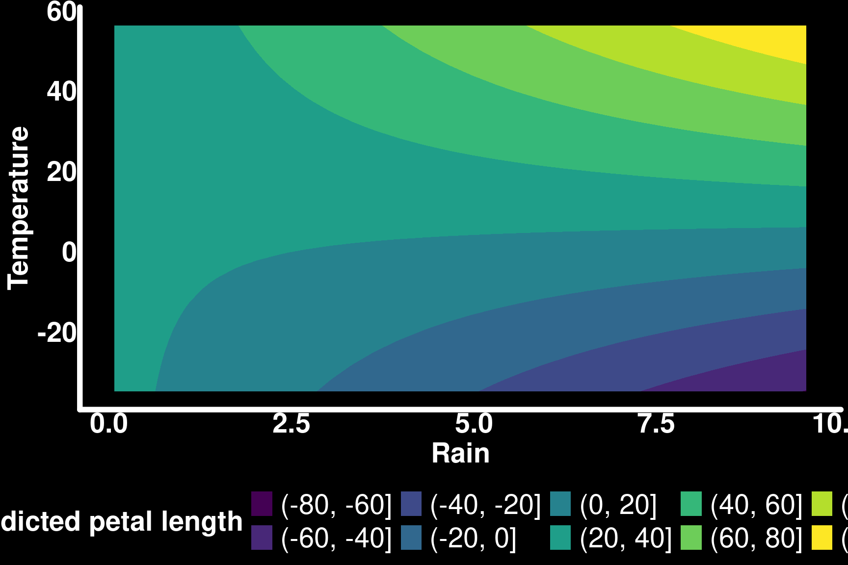
Response surfaces — use with caution
Code
predictions(mod_flower_1,newdata =datagrid(temp_centered =seq(min(flower_measurements_1$temp_centered),max(flower_measurements_1$temp_centered), length.out =30),rain_centered =seq(min(flower_measurements_1$rain_centered),max(flower_measurements_1$rain_centered), length.out =30) )) |>as_tibble() |>mutate(rain = rain_centered +mean(rain), temp = temp_centered +mean(temperature)) |>ggplot(aes(x = rain, y = temp, z = estimate)) +stat_contour_filled() +labs(x ="Rain", y ="Temperature", fill ="Predicted petal length")
Contour bins are arbitrary and hide uncertainty — good for exploration, risky for publication-quality inference. Prefer line-and-ribbon plots when you can.
🧪 Exercise 3
Using mod_flower_1:
Compute the slope of temperature across the observed range of rain (mirror the rain-across-temperature plot above).
At what value of rain does the temperature effect become non-significant (CI crosses zero), if at all?
Rewrite the research question this model could answer as a single sentence, identifying which variable is the exposure and which is the moderator.
(~7 minutes)
Interactions beyond the mean: distributional regression
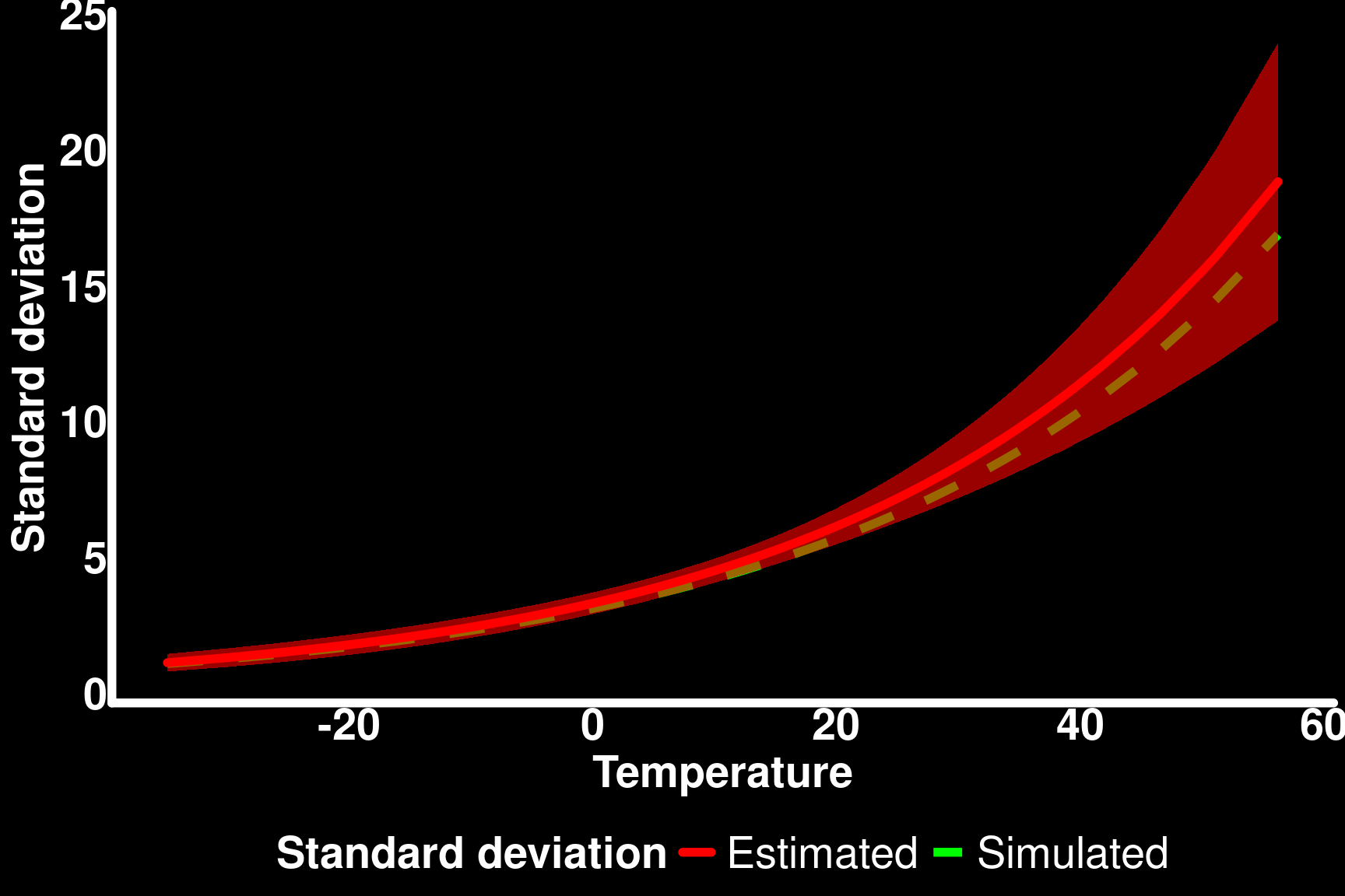
Interactions don’t have to act only on the average response. glmmTMB’s dispformula lets predictors affect the standard deviation too — useful when variance itself is ecologically meaningful (e.g., reduced trait variance under stress).
predictions(mod_flower_2, newdata = flower_measurements_2, type ="disp") |>as_tibble() -> pred_sd_temptrue_sd_temp <- flower_measurements_2 |>mutate(true_sd =exp(log_sd_intercept + log_sd_temp_slope * temp_centered))ggplot() +geom_line(data = true_sd_temp,aes(x = temp_centered +mean(temperature), y = true_sd, color ="Simulated"),linewidth =2, linetype ="dashed") +geom_ribbon(data = pred_sd_temp,aes(ymin = conf.low, ymax = conf.high, x = temp_centered +mean(temperature)),fill ="red", alpha =0.6) +geom_line(data = pred_sd_temp,aes(x = temp_centered +mean(temperature), y = estimate, color ="Estimated"),linewidth =2, lineend ="round") +scale_color_manual(values =c("Simulated"="green", "Estimated"="red"), name ="Standard deviation") +labs(x ="Temperature", y ="Standard deviation")
Recovered vs. simulated standard deviation of petal length.
type = "disp" retrieves predictions/slopes for the dispersion sub-model, exactly as type = "conditional" does for the mean.
🧪 Exercise 4 (challenge)
Extend mod_flower_2 by adding rain_centered and a temp_centered * rain_centered interaction to both the conditional formula and the dispformula.
Fit the model on simulated data of your own design (or reuse the logic from flower_measurements_2, adding a rain effect and interaction term on the log-sd scale).
Produce one plot showing how the effect of rain on the standard deviation of petal length changes across temperature.
In plain language, describe a real ecological scenario (not necessarily plants) where an interaction on variance, rather than the mean, would be the interesting finding.
(~10 minutes — this is open-ended; there’s no single correct answer)
Part 2 takeaways
With two numerical predictors, the interaction coefficient is the rate of change of one slope per unit of the other — not a separate slope for each group
Centering predictors makes main-effect coefficients interpretable as “effect at average conditions”
Plot slopes across the moderator’s range, not just the coefficient table
Five-number-summary prediction plots are usually more honest than response surfaces (they retain uncertainty)
Interactions can act on variance, not just the mean, via distributional regression (dispformula)
Wrap-up and further reading
Full write-ups with additional detail and 3D visualizations: Part 1, Part 2
A planned Part 3 will extend this material to non-Gaussian GLMs (non-linear link functions) and Part 4 to GAMs
Exercise solutions (instructor notes)
Exercise 1
mod_mass_true <- glmmTMB(weight ~ sex * snow_depth, data = bighorn_population, family = gaussian())
Male slope = snow_depth coefficient + sexmale:snow_depth coefficient
A naive pooled model would show a positive (or attenuated) relationship due to Simpson’s Paradox: sex confounds both snow exposure and baseline weight, so ignoring it would lead a manager to underestimate (or misjudge the direction of) the harm of a harsh winter.
Exercise 2
Uncorrected avg_slopes() on the biased sample is pulled toward the male slope (weaker effect) because males are overrepresented
Corrected version (using newdata_balanced) should land closer to mean(c(male_loss, female_loss))
Without a known true ratio, you would need an independent, unbiased estimate of population sex ratio (e.g., aerial survey, camera trap monitoring not subject to the same capture bias) to justify reweighting
Exercise 3
Mirror the code from the “slope across the range of the moderator” slide, swapping the roles of temp_centered and rain_centered
Answer depends on the random seed / simulated draw — have students report their own CI crossing point
Example framing: “Does the effect of temperature (exposure) on petal length depend on rainfall (moderator)?”