required_pkgs <- c("tidyverse", "glmmTMB", "marginaleffects", "patchwork", "GGally", "distributional", "TMB", "Matrix")

# Reinstalling Matrix/TMB/glmmTMB together (rather than one at a time) avoids the
# most common cause of glmmTMB load failures: an ABI mismatch between glmmTMB's
# compiled code and the Matrix/TMB versions it was linked against.
missing_pkgs <- required_pkgs[!vapply(required_pkgs, requireNamespace, logical(1), quietly = TRUE)]

if (length(missing_pkgs) > 0) {
  install.packages(missing_pkgs)
}

# Verify glmmTMB actually loads and can fit a trivial model - this is the step
# that catches ABI mismatches that "successful" installation can still leave behind.
glmmtmb_ok <- tryCatch({
  library(glmmTMB)
  test_fit <- glmmTMB(mpg ~ wt, data = mtcars)
  TRUE
}, error = function(e) {
  message("glmmTMB failed to load/fit: ", conditionMessage(e))
  FALSE
})

if (!glmmtmb_ok) {
  message("Reinstalling TMB and glmmTMB from source to resolve a likely ABI mismatch...")
  install.packages(c("TMB", "glmmTMB"), type = "source")

  # Re-check after the source reinstall
  glmmtmb_ok <- tryCatch({
    library(glmmTMB)
    glmmTMB(mpg ~ wt, data = mtcars)
    TRUE
  }, error = function(e) {
    message("Still failing: ", conditionMessage(e))
    message("If this persists, check that you have a working C++ compiler installed ",
            "(Rtools on Windows, Xcode command line tools on macOS), then restart R and re-run this chunk.")
    FALSE
  })
}

stopifnot("glmmTMB did not install/load successfully - see messages above" = glmmtmb_ok)Before you start
Run the chunk below once to install everything you need. It’s written to avoid the most common glmmTMB installation failures:
- Binary vs. source mismatch:
glmmTMBlinks againstTMBandMatrix, which must be built with compatible ABI versions. Installing all three together from the same repository snapshot (rather than upgrading one in isolation) avoids “package was installed with a different version” load-time errors. - Stale compiled objects after an R or
Matrixupgrade: if you’ve upgraded R recently and see an error likeError: package or namespace load failed for 'glmmTMB' ... unable to load shared object, reinstallingTMBandglmmTMBfrom source with--no-multiarch(viainstall.packages(type = "source")) usually fixes it. - Missing compiler toolchain: source installs of
TMB/glmmTMBneed a working C++ compiler. On Windows this means Rtools; on macOS, Xcode command line tools. The check below tells you if compilation is unavailable before you hit a cryptic error.
Setup
Run this at the start of every session (after the install chunk above has succeeded once).
library(tidyverse)       # Data manipulation and plotting
library(glmmTMB)         # Generalized linear (mixed) models
library(marginaleffects) # Compute marginal/conditional effects
library(patchwork)       # Combine multiple plots
library(GGally)          # Pairwise plots
library(distributional)  # Simulate mixture/gamma/normal distributions (Part 3)

theme_set(theme_minimal(base_size = 14))

set.seed(4127)
Coding style & functions used throughout
Before diving into the case studies, here’s a quick reference for the conventions and workhorse functions used repeatedly in this handout.
The native pipe, |>. Wherever you see data |> mutate(...) |> ggplot(...), read it left-to-right as “take data, and then apply mutate(), and then pass the result to ggplot()”. It’s equivalent to nesting the calls (ggplot(mutate(data, ...))), just easier to read and edit in sequence. We use the base-R pipe (|>), not the older magrittr pipe (%>%) — for our purposes here they behave the same way.
Simulating data with tibble() and random-draw functions. Every case study starts by simulating data rather than loading a real dataset. We pick “true” parameter values (an intercept, one or more slopes) up front, then generate observations from a known random process:
rnorm(n, mean, sd)— draws from a Normal distribution (continuous outcomes, e.g. weight, petal length)rbinom(n, size = 1, prob)— draws from a Bernoulli/Binomial distribution (presence/absence outcomes)rpois(n, lambda)— draws from a Poisson distribution (count outcomes, e.g. abundance)runif(n, min, max)— draws from a Uniform distribution (often used to simulate a predictor, not an outcome)
Simulating this way means we know the ground truth (the exact intercept and slopes used to generate the data), so we can directly check whether a fitted model recovers it — a habit worth carrying into your own work whenever you want to sanity-check a modeling approach before applying it to real data.
Fitting models with glmmTMB(). Our model-fitting workhorse throughout is glmmTMB(response ~ predictors, data = ..., family = ...). Key things to know:
y ~ x1 * x2expands toy ~ x1 + x2 + x1:x2— main effects for both predictors and their interaction, all in one shorthandfamily = gaussian()for continuous outcomes,binomial(link = "logit")for presence/absence,poisson(link = "log")for countsdispformula = ~ xlets predictors affect the variance of the outcome, not just its mean (used in the distributional-regression section of Part 2)
The marginaleffects package. Raw model coefficients (from summary()) are often not the quantity you actually want to report — especially with interactions or non-linear link functions. marginaleffects converts coefficients into direct, interpretable answers:
predictions()— the model-implied value of the outcome at specific covariate values (a conditional prediction)avg_predictions()— the same, but averaged over a distribution of covariate values (a marginal prediction)slopes()— the model-implied effect (derivative/slope) of one predictor on the outcome, at specific covariate valuesavg_slopes()— the same, averaged over a distribution of covariate valuesdatagrid(...)— builds the covariate grid at whichpredictions()/slopes()are evaluated; arguments can be fixed values, functions likemeanorfivenum(the five-number summary), or vectors of valuesby = "group"— instead of collapsing (averaging) over a variable, keep results broken out by its levelshypotheses(hypothesis = "b1 - b2 = 0")— tests linear combinations of estimates, e.g. “is the slope for group A different from the slope for group B?”
set.seed(). Called once near the top of each script (or before an exercise you want to be able to compare answers on) so that “random” simulation is actually reproducible — running the same code twice gives identical numbers. If your results differ from a classmate’s despite identical code, check whether you both used the same seed at the same point in the script.
Part 1 — Categorical × Numerical Interactions
Case study: Bighorn sheep
Ram Mountain, Alberta. Question: how does winter snow depth relate to spring mass in Bighorn sheep, and does it differ by sex? Males and females segregate in winter — females use lower, less snowy habitat.
n_individuals_population <- 1000
sexes <- c("male", "female")
male_intercept <- 220; female_intercept <- 180
sd_weight <- 15
male_loss <- -0.8; female_loss <- -2.5

bighorn_population <- tibble(
  sex = rep(sexes, n_individuals_population / length(sexes)),
  snow_depth = runif(n_individuals_population,
    min = ifelse(sex == "male", 35, 0),
    max = ifelse(sex == "male", 70, 35)
  ),
  weight = rnorm(n_individuals_population,
    mean = ifelse(sex == "male",
      male_intercept + male_loss * snow_depth,
      female_intercept + female_loss * snow_depth),
    sd = sd_weight
  )
)
Built-in features: different intercepts, different slopes, and different snow-depth distributions by sex.
Simpson’s Paradox
ggplot(bighorn_population, aes(x = snow_depth, y = weight)) +
  geom_point(aes(color = sex)) +
  geom_smooth(method = "lm", se = FALSE, color = "red", linewidth = 1)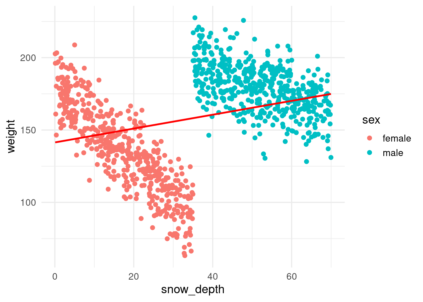
Pooled: snow depth looks positively associated with weight — even though both sexes lose weight with more snow.
ggplot(bighorn_population, aes(x = snow_depth, y = weight, color = sex)) +
  geom_point() +
  geom_smooth(method = "lm", se = FALSE)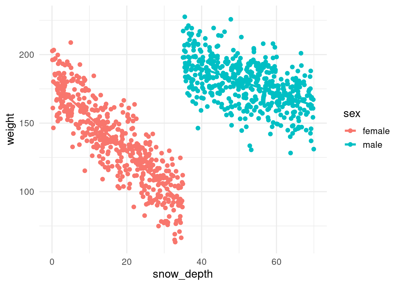
🧪 Exercise 1
Using bighorn_population:
- Fit
weight ~ sex * snow_depthwithglmmTMB(). Call itmod_mass_true. - From the summary, identify which coefficient represents the male slope of snow depth. (Hint: it’s not printed directly — you have to add two rows together.)
- In one sentence, explain why a naive
weight ~ snow_depthmodel (ignoring sex) would mislead a manager trying to understand the effect of a harsh winter.
Sampling from the population
In practice we can’t measure everyone. Two sampling scenarios:
- Scenario 1: balanced trap, 50 males / 50 females
- Scenario 2: biased trap, 80 males / 20 females
n_individuals <- 100
bighorn_mass_1 <- bighorn_population |>
  group_by(sex) |>
  slice_sample(n = n_individuals / 2, replace = FALSE) |>
  ungroup()

mod_mass_1 <- glmmTMB(weight ~ sex * snow_depth,
                       data = bighorn_mass_1, family = gaussian())
summary(mod_mass_1)$coefficients$cond
Estimate Std. Error z value Pr(>|z|)
(Intercept) 180.252394 4.5758581 39.392042 0.000000e+00
sexmale 49.686455 11.6121023 4.278851 1.878606e-05
snow_depth -2.485942 0.2124809 -11.699604 1.280491e-31
sexmale:snow_depth 1.534424 0.2937494 5.223580 1.754970e-07
attr(,"ddf")
[1] "asymptotic"Reading the coefficients:
- Intercept: female weight at snow_depth = 0
- sexmale: male − female intercept difference
- snow_depth: female slope
- sexmale:snow_depth: male − female slope difference
Q1: Do sexes differ in spring mass?
predictions(mod_mass_1, by = "sex")
    sex Estimate Std. Error    z Pr(>|z|)   S 2.5 % 97.5 %
 female      132       2.06 64.2   <0.001 Inf   128    137
 male        181       2.06 87.6   <0.001 Inf   177    185

Type: responsepredictions(mod_mass_1, by = "sex") |>
hypotheses(hypothesis = "b1 - b2 = 0")
 Hypothesis Estimate Std. Error     z Pr(>|z|)     S 2.5 % 97.5 %
    b1-b2=0    -48.3       2.92 -16.6   <0.001 202.2 -54.1  -42.6
Q2: Does snow depth affect mass equally by sex?
slopes(mod_mass_1, variables = "snow_depth", by = "sex", vcov = TRUE) |>
  ggplot(aes(x = estimate, xmax = conf.high, xmin = conf.low, y = sex, color = sex)) +
  geom_pointrange(size = 1) +
  theme(legend.position = "none")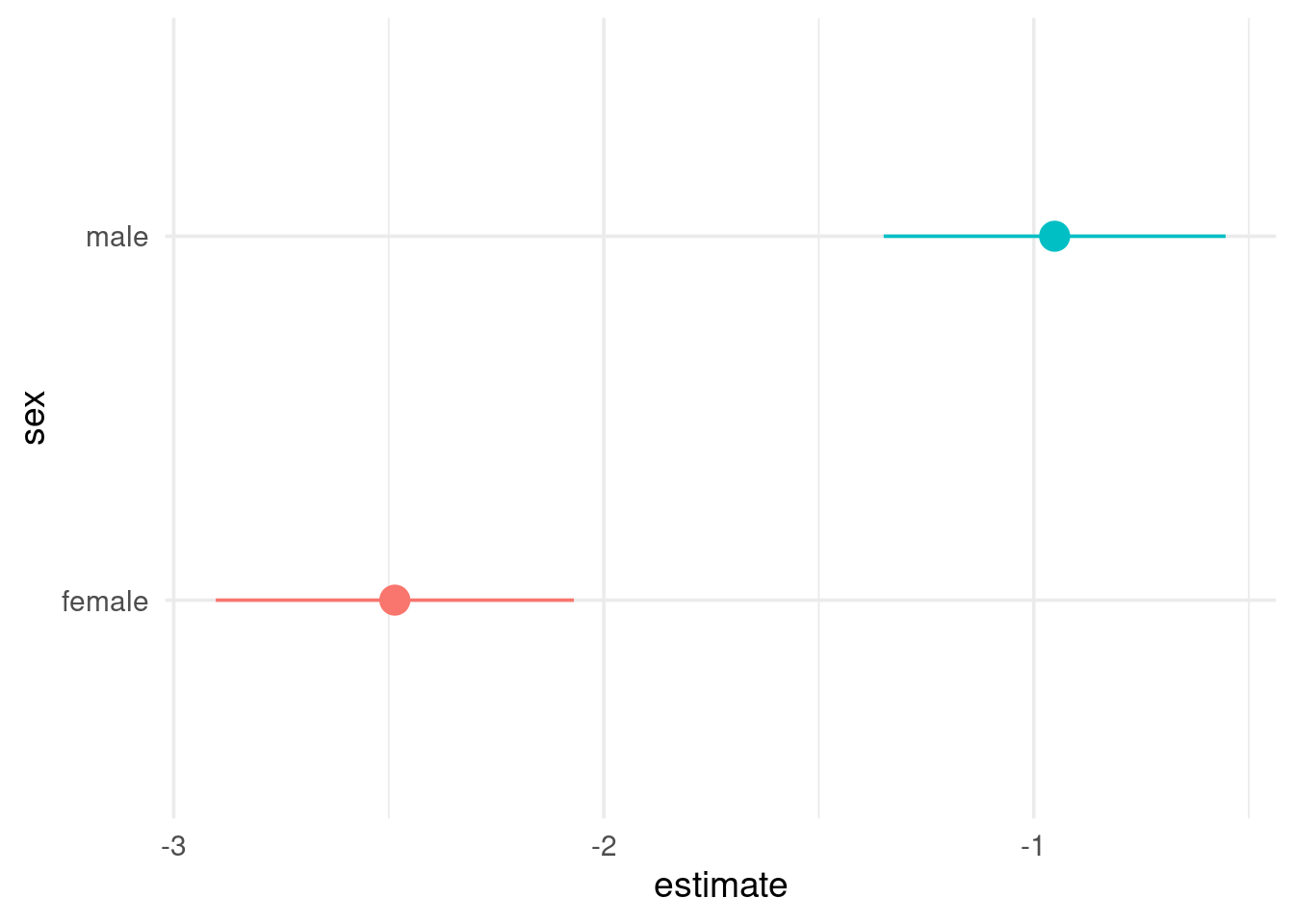
slopes(mod_mass_1, variables = "snow_depth", by = "sex", vcov = TRUE) |>
  hypotheses(hypothesis = "b1 - b2 = 0")
 Hypothesis Estimate Std. Error     z Pr(>|z|)    S 2.5 % 97.5 %
    b1-b2=0    -1.53      0.294 -5.22   <0.001 22.4 -2.11 -0.959
Q3: What’s the population-average slope?
avg_slopes() computes the slope for every observation, then averages:
avg_slopes(mod_mass_1, variables = "snow_depth", vcov = TRUE)
 Estimate Std. Error     z Pr(>|z|)     S 2.5 % 97.5 %
    -1.72      0.147 -11.7   <0.001 102.7 -2.01  -1.43

Term: snow_depth
Type: response
Comparison: dY/dX
Scenario 2: biased sampling (80% male)
bighorn_mass_2 <- bind_rows(
  bighorn_population |> filter(sex == "male") |> slice_sample(n = 80),
  bighorn_population |> filter(sex == "female") |> slice_sample(n = 20)
)
mod_mass_2 <- glmmTMB(weight ~ sex * snow_depth, data = bighorn_mass_2, family = gaussian())
avg_slopes(mod_mass_2, variables = "snow_depth", vcov = TRUE)
 Estimate Std. Error    z Pr(>|z|)    S 2.5 % 97.5 %
    -1.27      0.161 -7.9   <0.001 48.3 -1.58 -0.954

Term: snow_depth
Type: response
Comparison: dY/dX
Conditional (by-sex) slopes stay close to truth. But the marginal slope is biased toward the overrepresented, weaker-effect sex (males).
Correcting for known sampling bias
If we know the true population sex ratio (50:50), we can average over a balanced newdata grid instead of our biased sample.
newdata_balanced <- bighorn_mass_2 |>
  group_by(sex) |>
  reframe(snow_depth = seq(min(snow_depth), max(snow_depth), length.out = 50)) |>
  ungroup()

avg_predictions(mod_mass_2, variables = "snow_depth", newdata = newdata_balanced) |>
  as_tibble() |> select(estimate, conf.low, conf.high) |> head(3)
# A tibble: 3 × 3
estimate conf.low conf.high
<dbl> <dbl> <dbl>
1 201. 190. 212.
2 140. 132. 149.
3 124. 113. 134.🧪 Exercise 2
Using mod_mass_2 (the biased sample model):
- Compute
avg_slopes()without correcting for sampling bias, and again with the balancednewdata_balancedgrid. - Which one is closer to the true average slope,
mean(c(male_loss, female_loss))? - Suppose instead you didn’t know the true sex ratio in the population — what additional data would you need to collect to justify a correction like this?
Part 2 — Numerical × Numerical Interactions
Case study: petal length
Simulated flowers; petal length as a function of temperature and rain, with an interaction. Predictors are mean-centered: the intercept becomes the predicted response at average conditions rather than at (biologically meaningless) zero temperature/rain.
n_flowers <- 200
temperature <- rnorm(n_flowers, mean = 10, sd = 15)
rain <- rgamma(n_flowers, shape = 2)
avg_petal_length <- 25.6; sd_petal_length <- 4.5
temperature_effect <- 0.4; rain_effect <- 0.9; interaction_effect <- 0.2

flower_measurements_1 <- tibble(
  temp_centered = temperature - mean(temperature),
  rain_centered = rain - mean(rain),
  petal_length = rnorm(n_flowers,
    mean = avg_petal_length +
      temperature_effect * temp_centered +
      rain_effect * rain_centered +
      interaction_effect * temp_centered * rain_centered,
    sd = sd_petal_length)
)

mod_flower_1 <- glmmTMB(petal_length ~ temp_centered * rain_centered,
                         data = flower_measurements_1)
summary(mod_flower_1)$coefficients$cond
Estimate Std. Error z value Pr(>|z|)
(Intercept) 25.6288031 0.28512980 89.88469 0.000000e+00
temp_centered 0.3978619 0.01753886 22.68460 6.358816e-114
rain_centered 0.8783765 0.20525261 4.27949 1.873219e-05
temp_centered:rain_centered 0.2104061 0.01379506 15.25228 1.589951e-52
attr(,"ddf")
[1] "asymptotic"Slope of one predictor at a single value of the other
# Effect of temperature when rain_centered = 0 (i.e., average rain)
slopes(mod_flower_1, newdata = datagrid(rain_centered = 0),
       variables = "temp_centered")
 rain_centered Estimate Std. Error    z Pr(>|z|)     S 2.5 % 97.5 %
             0    0.398     0.0175 22.7   <0.001 376.0 0.363  0.432

Term: temp_centered
Type: response
Comparison: dY/dX
This matches the temp_centered coefficient directly — because rain is centered, “at rain = 0” means “at average rain.”
Slope across the range of the moderator
slopes_by_temp <- slopes(mod_flower_1,
  newdata = datagrid(temp_centered = seq(min(flower_measurements_1$temp_centered),
                                          max(flower_measurements_1$temp_centered), length.out = 30)),
  variables = "rain_centered", by = "temp_centered")

slopes_by_temp |>
  ggplot() +
  geom_hline(yintercept = 0, color = "blue", linetype = 2) +
  geom_ribbon(aes(x = temp_centered + mean(temperature), ymin = conf.low, ymax = conf.high),
    alpha = 0.4, fill = "lightgrey") +
  geom_line(aes(x = temp_centered + mean(temperature), y = estimate), linewidth = 1) +
  labs(y = "Effect of rain on petal length", x = "Temperature values")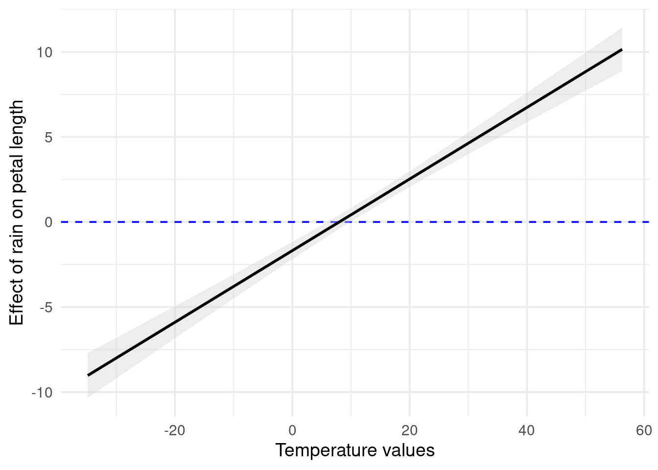
The interaction coefficient is exactly the slope of this line — how much the effect of rain changes per unit of temperature.
Visualizing predictions at chosen moderator values
Common choice: the five-number summary of the moderator.
predictions(mod_flower_1,
  newdata = datagrid(
    temp_centered = seq(min(flower_measurements_1$temp_centered),
                         max(flower_measurements_1$temp_centered), length.out = 30),
    rain_centered = fivenum
  )) |>
  as_tibble() |>
  mutate(rain = round(rain_centered + mean(rain), 2)) |>
  ggplot() +
  geom_line(aes(y = estimate, x = temp_centered + mean(temperature), color = as.factor(rain))) +
  geom_ribbon(aes(ymin = conf.low, ymax = conf.high,
                  x = temp_centered + mean(temperature), fill = as.factor(rain)), alpha = 0.2) +
  labs(y = "Predicted petal length", x = "Temperature", color = "Rain", fill = "Rain")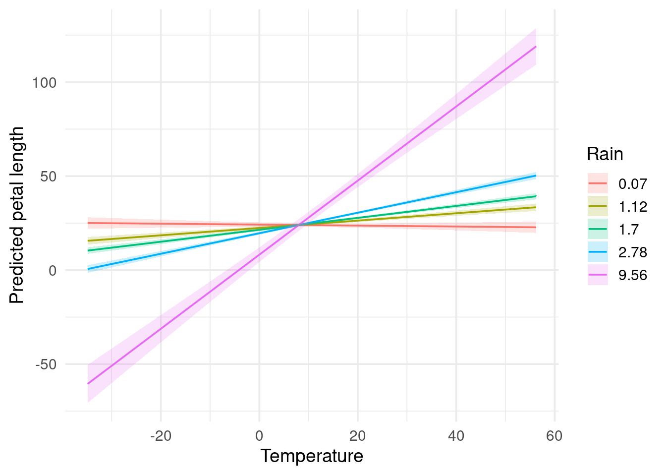
🧪 Exercise 3
Using mod_flower_1:
- Compute the slope of temperature across the observed range of rain (mirror the rain-across-temperature plot above).
- At what value of rain does the temperature effect become non-significant (CI crosses zero), if at all?
- Rewrite the research question this model could answer as a single sentence, identifying which variable is the exposure and which is the moderator.
Interactions beyond the mean: distributional regression
Interactions don’t have to act only on the average response. glmmTMB’s dispformula lets predictors affect the standard deviation too — useful when variance itself is ecologically meaningful (e.g., reduced trait variance under stress).
log_sd_intercept <- log(sd_petal_length)
log_sd_temp_slope <- 0.03

flower_measurements_2 <- tibble(
  temp_centered = temperature - mean(temperature),
  rain_centered = rain - mean(rain),
  petal_length = rnorm(n_flowers,
    mean = avg_petal_length + temperature_effect * temp_centered,
    sd = exp(log_sd_intercept + log_sd_temp_slope * temp_centered))
)

mod_flower_2 <- glmmTMB(petal_length ~ temp_centered,
                         dispformula = ~ temp_centered,
                         data = flower_measurements_2)
pred_sd_temp <- predictions(mod_flower_2, newdata = flower_measurements_2, type = "disp") |>
as_tibble()
true_sd_temp <- flower_measurements_2 |>
mutate(true_sd = exp(log_sd_intercept + log_sd_temp_slope * temp_centered))
ggplot() +
geom_line(data = true_sd_temp,
aes(x = temp_centered + mean(temperature), y = true_sd, color = "Simulated"),
linewidth = 1, linetype = "dashed") +
geom_ribbon(data = pred_sd_temp,
aes(ymin = conf.low, ymax = conf.high, x = temp_centered + mean(temperature)),
fill = "red", alpha = 0.3) +
geom_line(data = pred_sd_temp,
aes(x = temp_centered + mean(temperature), y = estimate, color = "Estimated"),
linewidth = 1) +
scale_color_manual(values = c("Simulated" = "darkgreen", "Estimated" = "red"), name = "Standard deviation") +
labs(x = "Temperature", y = "Standard deviation")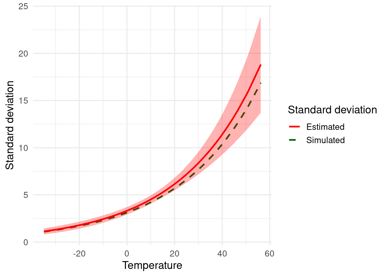
type = "disp" retrieves predictions/slopes for the dispersion sub-model, exactly as type = "conditional" does for the mean.
🧪 Exercise 4 (challenge)
Extend mod_flower_2 by adding rain_centered and a temp_centered * rain_centered interaction to both the conditional formula and the dispformula.
- Fit the model on simulated data of your own design (or reuse the logic from
flower_measurements_2, adding a rain effect and interaction term on the log-sd scale). - Produce one plot showing how the effect of rain on the standard deviation of petal length changes across temperature.
- In plain language, describe a real ecological scenario (not necessarily plants) where an interaction on variance, rather than the mean, would be the interesting finding.
Part 3 — Link Functions Create Implicit Interactions
Non-linear link functions (logit, log, …) introduce a second, implicit source of interaction: even a model with no interaction term at all can show predictors whose response-scale effect depends on the values of other predictors. This happens because the link function bends a straight line (on the link scale) into a curve (on the response scale).
Case study: species occurrence
Simulated presence/absence of a species across 200 plots, as a function of tree cover, rain, and temperature — no interaction terms, fit with a binomial GLM (logit link).
n_plots <- 200
tree_cover <- dist_mixture(dist_beta(4, 0.8), dist_beta(0.8, 4), weights = c(0.5, 0.5))
avg_yearly_rain <- dist_gamma(shape = 3, rate = 0.7)
avg_yearly_temp <- dist_normal(mu = 20, sd = 10)

occurence_intercept <- plogis(-3)
occurence_tree_effect <- 0.45
occurence_rain_effect <- 0.01
occurence_temp_effect <- 0.01

occ_data <- tibble(
  tree_cov = generate(tree_cover, n_plots),
  rain = generate(avg_yearly_rain, n_plots),
  temp = generate(avg_yearly_temp, n_plots)
) |>
  unnest(everything()) |>
  mutate(occurence = rbinom(n_plots, size = 1,
    prob = occurence_intercept +
      occurence_tree_effect * tree_cov +
      occurence_rain_effect * rain +
      occurence_temp_effect * temp))
mod_1 <- glmmTMB(occurence ~ tree_cov + rain + temp, family = binomial(link = "logit"), data = occ_data)
summary(mod_1)$coefficients$cond Estimate Std. Error z value Pr(>|z|)
(Intercept) -1.57990035 0.49404071 -3.197915 1.384249e-03
tree_cov 1.89295895 0.43249936 4.376790 1.204398e-05
rain 0.06558535 0.05850909 1.120943 2.623121e-01
temp 0.02060719 0.01559519 1.321381 1.863742e-01
attr(,"ddf")
[1] "asymptotic"We simulated the effect of tree cover to be 0.45 on the probability scale, but the model reports ~1.87. That’s not an error — it’s reporting the coefficient on the log-odds scale, not the probability scale.
The logit link bends a line into an S-shape
tibble(log_odds = seq(-6, 6, length.out = 400)) |>
  mutate(probability = plogis(log_odds)) |>
  ggplot(aes(x = log_odds, y = probability)) +
  geom_line(linewidth = 1) +
  labs(x = "log-odds scale (what the coefficient describes)",
       y = "probability scale (what we care about)")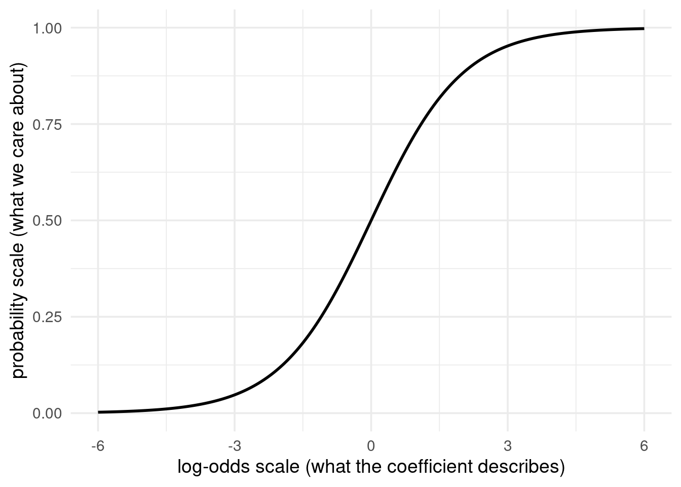
Near the middle (p ≈ 0.5) the curve is steep: a small log-odds push moves probability a lot. Near the ends (p ≈ 0 or 1) the curve flattens: the same push barely moves probability.
From log-odds to probability, by hand
The derivative of the inverse-logit gives the conversion: if \(\eta\) is the log-odds and \(p = \text{logit}^{-1}(\eta)\),
\[\frac{dp}{dX} = p(1-p) \times \beta\]
beta_tree <- fixef(mod_1)$cond["tree_cov"]
eta <- predict(mod_1, newdata = datagrid(model = mod_1, temp = mean(occ_data$temp),
                                          rain = mean(occ_data$rain)), type = "link")
p <- plogis(eta)
p * (1 - p) * beta_tree  # compare to slopes() below, and to our simulated 0.45
tree_cov
0.4727553 marginaleffects does this same conversion for us directly:
slopes(mod_1, variables = "tree_cov",
       newdata = datagrid(temp = mean(occ_data$temp), rain = mean(occ_data$rain)))
 temp rain Estimate Std. Error    z Pr(>|z|)    S 2.5 % 97.5 %
 19.7 4.24    0.473      0.108 4.38   <0.001 16.3 0.261  0.684

Term: tree_cov
Type: response
Comparison: dY/dX
The implicit interaction, visualized
slopes(mod_1, variables = "tree_cov", newdata = datagrid(temp = fivenum, rain = fivenum)) |>
  ggplot() +
  geom_pointrange(aes(x = estimate, xmin = conf.low, xmax = conf.high, y = 1)) +
  geom_vline(xintercept = occurence_tree_effect, alpha = .8) +
  facet_grid(rain ~ temp) +
  theme(axis.title.y = element_blank(), axis.text.y = element_blank())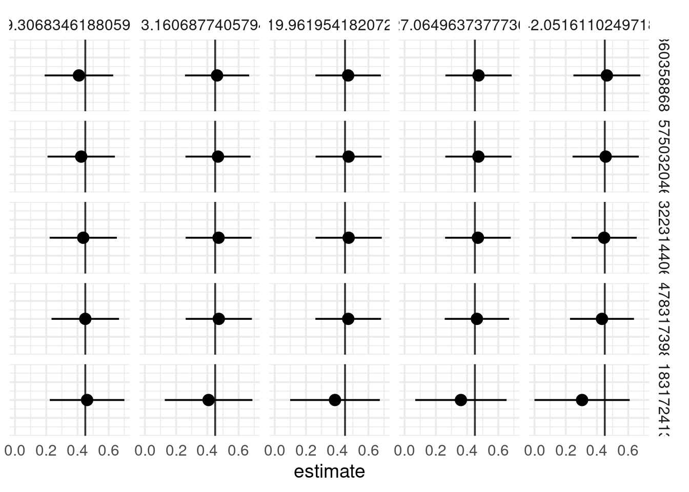
Because the amount of “bending” depends on where you are on the S-curve, tree cover’s probability-scale effect depends on rain and temp too — even though we never told the model to include that interaction. Whether an interaction “exists” can depend on which scale you look at (additive/probability vs. multiplicative/log-odds) — see Spake et al. (2023) for more on this “Type-D” error.
🧪 Exercise 5
Using mod_1:
- Compute the probability-scale slope of
tree_covat the minimum and maximum observed values ofrainandtemp(four combinations total, viadatagrid()). - Which combination gives the smallest slope? Which gives the largest? Relate your answer to where those combinations fall on the S-curve.
- In one sentence, explain why reporting only the raw
summary(mod_1)coefficient fortree_covwould be misleading to a reader who cares about probability of occurrence.
Case study: species abundance
The same phenomenon shows up with count data. Abundance (when present) as a function of the same three predictors, fit with a Poisson GLM (log link), again no interaction terms.
abundance_intercept <- exp(1)
abundance_tree_effect <- 4.5
abundance_rain_effect <- 0.1
abundance_temp_effect <- 0.1

abund_data <- tibble(
  tree_cov = generate(tree_cover, n_plots),
  rain = generate(avg_yearly_rain, n_plots),
  temp = generate(avg_yearly_temp, n_plots)
) |>
  unnest(everything()) |>
  mutate(abundance = rpois(n_plots, lambda =
    abundance_intercept +
    abundance_tree_effect * tree_cov +
    abundance_rain_effect * rain +
    abundance_temp_effect * temp))

mod_2 <- glmmTMB(abundance ~ tree_cov + rain + temp, family = poisson(link = "log"), data = abund_data)
summary(mod_2)$coefficients$cond
Estimate Std. Error z value Pr(>|z|)
(Intercept) 1.22278842 0.088646929 13.7939175 2.772841e-43
tree_cov 0.71228337 0.075917457 9.3823396 6.452479e-21
rain 0.01054384 0.011186717 0.9425318 3.459204e-01
temp 0.01541014 0.002750491 5.6026867 2.110545e-08
attr(,"ddf")
[1] "asymptotic"The log-scale tree_cov coefficient is ~0.73, not 4.5.
The log link bends a line into an exponential curve
tibble(log_count = seq(-2, 6, length.out = 400)) |>
  mutate(count = exp(log_count)) |>
  ggplot(aes(x = log_count, y = count)) +
  geom_line(linewidth = 1) +
  labs(x = "log scale (what the coefficient describes)", y = "count scale (what we care about)")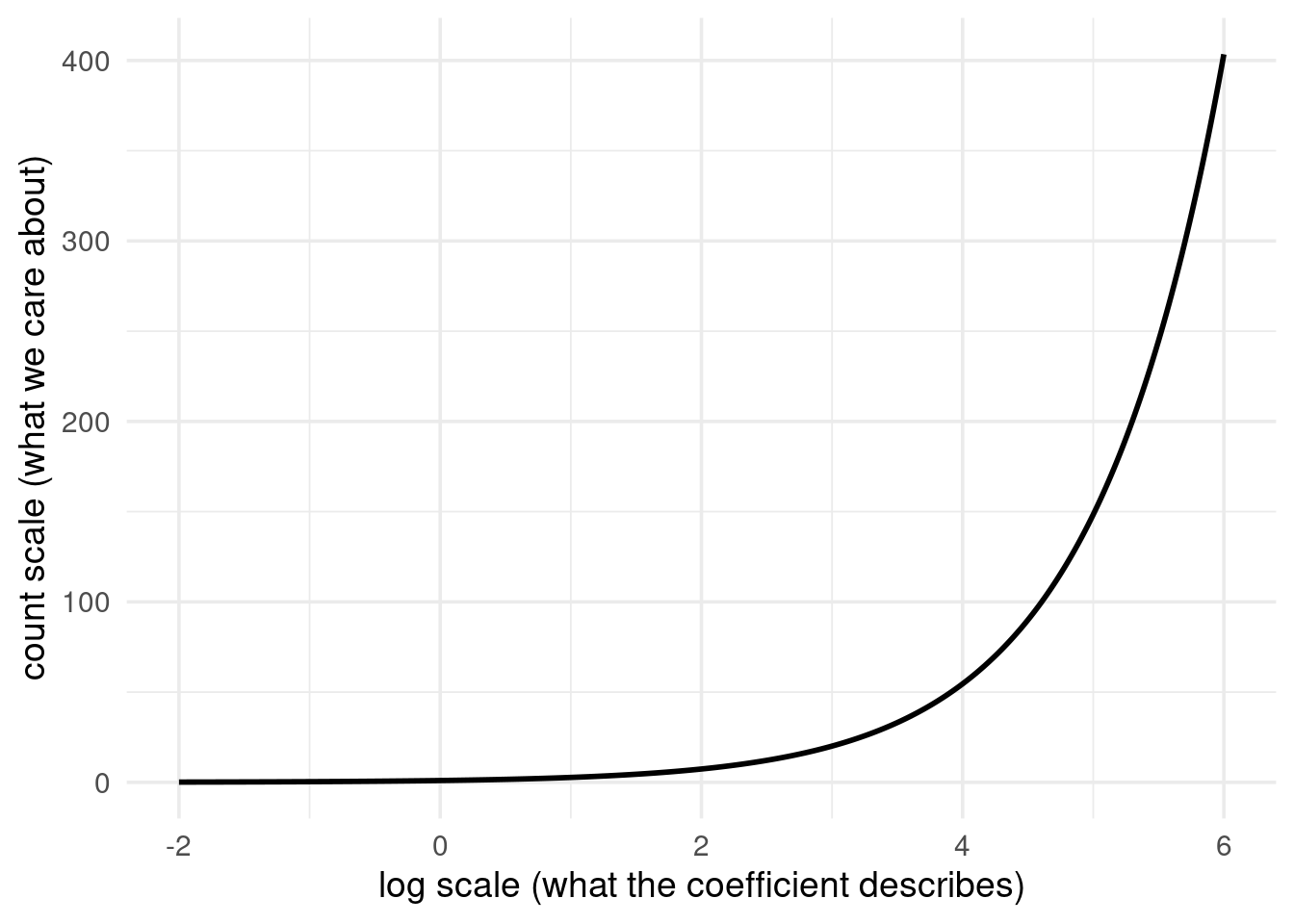
The local rate of change on the count scale is \[\lambda \cdot \beta\] (the expected count itself, times the log-scale coefficient) — the count-scale analogue of \[p(1-p)\cdot\beta\].
Two ways to report a log-link coefficient
- Rate ratio (\[e^\beta\]): a constant multiplicative effect, valid everywhere — “each unit increase in tree cover multiplies expected abundance by this factor, regardless of rain or temp”
- Local slope (\[\lambda \cdot \beta\]): an additive, count-scale effect (“this many more individuals”), but only valid near the specific covariate values used
exp(fixef(mod_2)$cond["tree_cov"]) # rate ratio: ~2.08, i.e. a ~108% increase per unit tree covertree_cov
2.038641 beta_tree_2 <- fixef(mod_2)$cond["tree_cov"]
eta_2 <- predict(mod_2, newdata = datagrid(model = mod_2, temp = mean(abund_data$temp),
rain = mean(abund_data$rain)), type = "link")
lambda <- exp(eta_2)
lambda * beta_tree_2 # local count-scale slope, close to our simulated 4.5tree_cov
4.966101 Both describe the same underlying model — pick the one that matches your audience (percent change vs. a concrete headcount).
🧪 Exercise 6
Using mod_2:
- Compute the rate ratio and the local count-scale slope for
temp, holdingrainat its minimum (a “drought” scenario) andtree_covat its mean. - Repeat holding
tree_covat a low vs. a high value (e.g., the 10th and 90th percentiles) — does the rate ratio change? Does the local slope? - Explain, in your own words, why one of these two summaries stays constant across
tree_covand the other doesn’t.
Further reading
- Full write-up with additional detail: Part 3 tutorial
marginaleffectsdocumentation: https://marginaleffects.com/- Spake et al. (2023), on interactions in GLMs: https://onlinelibrary.wiley.com/doi/full/10.1111/brv.12939